Capital Structure
Chapter 16. Capital Structure. Chapter Outline. 16.1 Capital Structure Choices 16.2 Capital Structure in Perfect Capital Markets 16.3 Debt and Taxes 16.4 Costs of Bankruptcy and Financial Distress 16.5 Optimal Capital Structure: The Tradeoff Theory

Capital Structure
E N D
Presentation Transcript
Chapter 16 Capital Structure
Chapter Outline 16.1 Capital Structure Choices 16.2 Capital Structure in Perfect Capital Markets 16.3 Debt and Taxes 16.4 Costs of Bankruptcy and Financial Distress 16.5 Optimal Capital Structure: The Tradeoff Theory 16.6 Additional Consequences of Leverage: Agency Costs and Information
Learning Objectives Examine how capital structures vary across industries and companies Understand why investment decisions, rather than financing decisions, fundamentally determine the value and cost of capital of the firm Describe how leverage increases the risk of the firm’s equity Demonstrate how debt can affect firm value through taxes and bankruptcy costs
Learning Objectives (cont’d) Show how the optimal mix of debt and equity trades off the costs (including financial distress costs) and benefits (including the tax advantage) of debt Analyze how debt can alter the incentives of managers to choose different projects and can be used as a signal to investors Weigh the many costs and benefits to debt that a manager must balance when deciding how to finance the firm’s investments
16.1 Capital Structure Choices When raising funds from outside investors, a firm must choose what type of security to issue and what capital structure to have.
16.1 Capital Structure Choices Capital structure The collection of securities a firm issues to raise capital from investors. Firms consider whether the securities issued: Will receive a fair price in the market Have tax consequences Entail transactions costs Change future investment opportunities
16.1 Capital Structure Choices A firm’s debt-to-value ratio is the fraction of the firm’s total value that corresponds to debt D / (E+D)
Figure 16.1 Debt-to-Value Ratio [D/(E + D)] for Select Industries
Figure 16.2 Capital Structures of Amazon.com and Barnes & Noble
16.2 Capital Structure in Perfect Capital Markets A perfect capital market is a market in which: Securities are fairly priced No tax consequences or transactions costs Investment cash flows are independent of financing choices
16.2 Capital Structure in Perfect Capital Markets Unlevered equity equity in a firm with no debt Levered equity equity in a firm that has debt outstanding Leverage will increase the risk of the firm’s equity and raise its equity cost of capital
16.2 Capital Structure in Perfect Capital Markets Modigliani and Miller (MM) with perfect capital markets In an unlevered firm, cash flows to equity equal the free cash flows from the firm’s assets. In a levered firm, the same cash flows are divided between debt and equity holders. The total to all investors equals the free cash flows generated by the firm’s assets.
Figure 16.3 Unlevered Versus Levered Cash Flows with Perfect Capital Markets
16.2 Capital Structure in Perfect Capital Markets MM Proposition I: In a perfect capital market, the total value of a firm is equal to the market value of the free cash flows generated by its assets and is not affected by its choice of capital structure. VL= E + D =VU (Eq. 16.1)
Table 16.1 Returns to Equity in Different Scenarios with and Without Leverage
Figure 16.4 Unlevered Versus Levered Returns with Perfect Capital Market
Example 16.1 The Risk and Return of Levered Equity Problem: Suppose you borrow only $6,000 when financing your coffee shop. According to Modigliani and Miller, what should the value of the equity be? What is the expected return?
Example 16.1 The Risk and Return of Levered Equity Solution: Plan: The value of the firm’s total cash flows does not change: it is still $30,000. Thus, if you borrow $6000, your firm’s equity will be worth $24,000. To determine its expected return, we will compute the cash flows to equity under the two scenarios . The cash flows to equity are the cash flows of the firm net of the cash flows to debt (repayment of principal plus interest).
Example 16.1 The Risk and Return of Levered Equity Execute: The firm will owe debt holders $6,000 1.05 = $6,300 in one year. Thus, the expected payoff to equity holders is $34,500 – $6,300 = $28,200, for a return of $28,200 / $24,000 – 1 = 17.5%.
Example 16.1 The Risk and Return of Levered Equity Evaluate: While the total value of the firm is unchanged, the firm’s equity in this case is more risky than it would be without debt, but less risky than if the firm borrowed $15,000. To illustrate, note that if demand is weak, the equity holders will receive $27,000 – $6,300 = $20,700, for a return of $20,700/$24,000 – 1 = – 13.75%.
Example 16.1 The Risk and Return of Levered Equity Evaluate (cont’d): Compare this return to – 10% without leverage and – 25% if the firm borrowed $15,000. As a result, the expected return of the levered equity is higher in this case than for unlevered equity (17.5% versus 15%), but not as high as in the previous example (17.5% versus 25% with more leverage).
Example 16.1a The Risk and Return of Levered Equity Problem: Suppose you borrow $50,000 when financing a coffee shop which is valued at $75,000. You expect to generate a cash flow of $75,000 at the end of the year if demand is weak, $84,000 if demand is as expected and $93,000 if demand is strong. Each scenario is equally likely. The current risk-free interest rate is 4%, and there’s an 8% risk premium for the risk of the assets. According to Modigliani and Miller, what should the value of the equity be? What is the expected return?
Example 16.1a The Risk and Return of Levered Equity Solution: Plan: The value of the firm’s total cash flows does not change: it is still $75,000 (expected cash flow of $84,000 discounted at 12%). Thus, if you borrow $50,000, your firm’s equity will be worth $25,000. To determine its expected return, we will compute the cash flows to equity under the two scenarios. The cash flows to equity are the cash flows of the firm net of the cash flows to debt (repayment of principal plus interest).
Example 16.1a The Risk and Return of Levered Equity Execute: The firm will owe debt holders $50,000 1.04 = $52,000 in one year. Thus, the expected payoff to equity holders is $84,000 – $52,000 = $32,000, for a return of $32,000 / $25,000 – 1 = 28%.
Example 16.1a The Risk and Return of Levered Equity Evaluate: While the total value of the firm is unchanged, the firm’s equity in this case is more risky than it would be without debt. To illustrate, if demand is weak, the equity holders will receive $75,000 – $52,000 = $23,000, for a return of $23,000/$25,000 – 1 = – 8%. If demand is strong, the equity holders will receive $93,000 – $52,000 = $41,000, for a return of $41,000/$25,000 – 1 = 64%. Without debt, equity holders expect to receive $84,000/75,000 – 1 = 12%.
Example 16.1b The Risk and Return of Levered Equity Problem: Suppose you borrow $25,000 when financing a coffee shop which is valued at $75,000. As in Example 16.1a, you expect to generate a cash flow of $75,000 at the end of the year if demand is weak, $84,000 if demand is as expected and $93,000 if demand is strong. Each scenario is equally likely. The current risk-free interest rate is 4%, and there’s an 8% risk premium for the risk of the assets. According to Modigliani and Miller, what should the value of the equity be? What is the expected return?
Example 16.1b The Risk and Return of Levered Equity Solution: Plan: The value of the firm’s total cash flows does not change: it is still $75,000 (the expected $84,000 cash flow discounted at 12%). Thus, if you borrow $25,000, your firm’s equity will be worth $50,000. To determine its expected return, we will compute the cash flows to equity under the two scenarios. The cash flows to equity are the cash flows of the firm net of the cash flows to debt (repayment of principal plus interest).
Example 16.1b The Risk and Return of Levered Equity Execute: The firm will owe debt holders $25,000 1.04 = $26,000 in one year. Thus, the expected payoff to equity holders is $84,000 – $26,000 = $58,000, for a return of $58,000 / $50,000 – 1 = 16%.
Example 16.1b The Risk and Return of Levered Equity Evaluate: While the total value of the firm is unchanged, the firm’s equity in this case is more risky than it would be without debt, but less risky than if the firm borrowed $50,000. To illustrate, if demand is weak, the equity holders will receive $75,000 – $26,000 = $49,000, for a return of $49,000/$50,000 – 1 = – 2%. If demand is strong, the equity holders will receive $93,000 – $26,000 = $67,000, for a return of $67,000/$50,000 – 1 = 34%.
16.2 Capital Structure in Perfect Capital Markets Homemade leverage Investors use leverage in their own portfolios to adjust firm’s leverage A perfect substitute for firm leverage in perfect capital markets.
16.2 Capital Structure in Perfect Capital Markets Leverage and the Cost of Capital Weighted average cost of capital (pretax) (Eq. 16.2)
16.2 Capital Structure in Perfect Capital Markets MM Proposition II: The cost of capital of levered equity: The Cost of Levered Equity Cost of levered equity equals the cost of unlevered equity plus a premium proportional to the debt-equity ratio. (Eq. 16.3)
Example 16.2 Computing the Equity Cost of Capital Problem: Suppose you borrow only $6,000 when financing your coffee shop. According to MM Proposition II, what will your firm’s equity cost of capital be?
Example 16.2 Computing the Equity Cost of Capital Solution: Plan: Because your firm’s assets have a market value of $30,000, by MM Proposition I the equity will have a market value of $24,000 = $30,000 – $6,000. We can use Eq. 16.3 to compute the cost of equity. We know the unlevered cost of equity is ru = 15%. We also know that rD is 5%.
Example 16.2 Computing the Equity Cost of Capital Evaluate: This result matches the expected return calculated in Example 16.1 where we also assumed debt of $6,000. The equity cost of capital should be the expected return of the equity holders.
Example 16.2a Computing the Equity Cost of Capital Problem: Referring back to Example 16.1a, suppose you borrow $50,000 when financing your coffee shop. According to MM Proposition II, what will your firm’s equity cost of capital be?
Example 16.2a Computing the Equity Cost of Capital Solution: Plan: Because your firm’s assets have a market value of $75,000, by MM Proposition I the equity will have a market value of $25,000 = $75,000 – $50,000. We can use Eq. 16.3 to compute the cost of equity. We know the unlevered cost of equity is ru = 12%. We also know that rD is 4%.
Example 16.2a Computing the Equity Cost of Capital Evaluate: This result matches the expected return calculated in Example 16.1a where we also assumed debt of $50,000. The equity cost of capital should be the expected return of the equity holders.
Example 16.2b Computing the Equity Cost of Capital Problem: Referring back to Example 16.1b, suppose you borrow $25,000 when financing your coffee shop. According to MM Proposition II, what will your firm’s equity cost of capital be?
Example 16.2b Computing the Equity Cost of Capital Solution: Plan: Because your firm’s assets have a market value of $75,000, by MM Proposition I the equity will have a market value of $50,000 = $75,000 – $25,000. We can use Eq. 16.3 to compute the cost of equity. We know the unlevered cost of equity is ru = 12%. We also know that rD is 4%.
Example 16.2b Computing the Equity Cost of Capital Evaluate: This result matches the expected return calculated in Example 16.1b where we also assumed debt of $25,000. The equity cost of capital should be the expected return of the equity holders.
16.3 Debt and Taxes Market imperfections can create a role for the capital structure. Corporate taxes: Corporations can deduct interest expenses. Reduces taxes paid Increases amount available to pay investors. Increases value of the corporation.
16.3 Debt and Taxes Consider the impact of interest expenses on taxes paid by Safeway, Inc. In 2008, Safeway had earnings before interest and taxes of $1.85 billion Interest expenses of $400 million Corporate tax rate is 35% Compare Safeway’s actual net income with what it would have been without debt.
Table 16.2 Safeway’s Income with and without Leverage, 2008 ($ millions) Total amount available to all investors is:
16.3 Debt and Taxes Interest Tax Shield The gain to investors from the tax deductibility of interest payments Interest Tax Shield = Corporate Tax Rate Interest Payments
Example 16.3 Computing the Interest Tax Shield Problem: Shown on the next slide is the income statement for E.C. Builders (ECB). Given its marginal corporate tax rate of 35%, what is the amount of the interest tax shield for DFB in years 2007 through 2010?