Chapter 6 The Revised Simplex Method
Chapter 6 The Revised Simplex Method. This method is a modified version of the Primal Simplex Method that we studied in Chapter 5.

Chapter 6 The Revised Simplex Method
E N D
Presentation Transcript
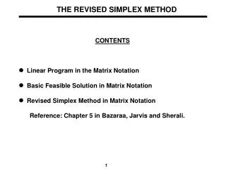
Chapter 6The Revised Simplex Method • This method is a modified version of the Primal Simplex Method that we studied in Chapter 5. • It is designed to exploit the fact that in many practical applications the coefficient matrix {aij} is very sparse, namely most of its elements are equal to zero.
Bottom line: • Don’t update all the columns of the simplex tableau: update only those columns that you need!
Standard Form • opt=max • ~ • bi ≥ 0 , • for all i.
Canonical Form As in the standard format, bi≥0 for all i.
System P (6.4)
After a number of Pivot Operations System P’
Observation • After any iteration of the simplex method the columns of the m basic variables comprise the columns of the mxm identity matrix. • The order in which these columns are arranged for this purpose is important. • This order is specified in the BV column of the simplex tableau.
6.2 The Transformation • How can we compute S’ from S ? • From Linear Algebra we know that any finite sequence of pivot operations is equivalent to (left) multiplication by a matrix. • In other words, S’ = TS • The question is then: T = ??????
What is T ??? • Observation 1: After any number of iterations of the simplex method, the columns of the coefficient matrix corresponding to the basic variables at that iteration, comprise the identity matrix. • Observation 2: Initially, the last m columns of the coefficient matrix comprise the identity matrix.
Analysis • If we group the columns of the basic variables into I and the nonbasic variables into D’, then S’ = [I,D’] • If we do the same for the initial matrix S, we have S = [B,D] where B is the matrix constructed from the columns of the initial matrix corresponding to the current basic variables.
Since S’ = TS, it follows that S’ = [I,D’] = TS = [TB,TD] hence I = TB from which we conclude that T = B-1
Notation: • IB = Indices of the basic elements (in canonical form) • ID = indices of the nonbasic variables in increasing order • cB = Initial cost vector of the basic variables • cD = Initial cost vector of the nonbasic variables
r = reduced costs vector • D = columns of the coefficient matrix in the initial simplex tableau corresponding to the current nonbasic variables.
Behind the Formula (NILN) • Each column of the coefficient matrix in the new tableau is equal to B-1 times the corresponding initial column, i.e new column = B-1 initial column • This is also true for the right-hand-side vector, i.e new RHS = B-1 initial RHS • Observe that the z-row is not included in this formulation (why?)
rD = correction • C’B = (0,0,...,0)
(NILN)But how do we compute B-1 ? • Bad news: • We have to compute it as we go along • Good News: • We do not have to compute it from scratch • Observation: S’ = B-1S = B-1 [M,I] = [B-1M,B-1I] = [B-1M,B-1] • Hence, B-1 is equal to the matrix comprising the last m columns of the LHS matrix.