Geomath Basics: Solving Geological Problems with Mathematics |
Learn about age-depth relationships, common geological variables, linear and non-linear equations, and polynomial functions in geology. Explore equations and interpretations for better understanding. |

Geomath Basics: Solving Geological Problems with Mathematics |
E N D
Presentation Transcript
Geology 351 - Geomath Basic Review tom.h.wilson tom.wilson@mail.wvu.edu Department of Geology and Geography West Virginia University Morgantown, WV
Chapter 1 Mathematics as a tool for solving geological problems The example presented on page 3 illustrates a simple age-depth relationship for unlithified sediments This equation is a quantitative statement of what we all have an intuitive understanding of - increased depth of burial translates into increased age of sediments. But as Waltham suggests - this is an approximation of reality. What does this equation assume about the burial process? Is it a good assumption?
where a=age, z=depth Example - if k = 1500 years/m calculate sediment age at depths of 1m, 2m and 5.3m. Repeat for k =3000 years/m Age = 1500 years 1m 2m 5.3m Age = 3000 years Age = 7950 years For k = 3000years/m Age = 3000 years Age = 6000 years Age = 15900 years
Chapter 2 - Common relationships between geological variables You probably recognized that the equation we started with is the equation of a straight line. The general equation of a straight line is
In this equation - which term is the slope and which is the intercept? In this equation - which term is the slope and which is the intercept? A more generalized representation of the age/depth relationship should include an intercept term -
If only the relative ages of the sediments are known, then for a given value of k (inverse deposition rate) we would have a family of possible lines defining age versus depth. What are the intercepts? Are all these curves realistic?
Consider the case for sediments actively deposited in a lake. Consider the significance of A0 in the following context If k is 1000 years/meter, what is the velocity that the lake bed moves up toward the surface? and If the lake is currently 15 meters deep, how long will it take to fill up?
The slope (k) does not change. We still assume that the thickness of the sediments continues to increase at the rate of 1 meter in 1000 years. What is the intercept? Hint: A must be zero when D is 15 meters
present day depth at age = 0. You should be able to show that A0 is -15,000 years. That means it will take 15,000 years for the lake to fill up. -15,000
Is this a good model? … we would guess that the increased weight of the overburden would squeeze water from the formation and actually cause grains to be packed together more closely. Thus meter thick intervals would not correspond to the same interval of time. Meter-thick intervals at greater depths would correspond to greater intervals of time.
We might also guess that at greater and greater depths the grains themselves would deform in response to the large weight of the overburden pushing down on each grain.
These compaction effects make the age-depth relationship non-linear. The same interval of depth D at large depths will include sediments deposited over a much longer period of time than will a shallower interval of the same thickness.
The relationship becomes non-linear. The line y=mx+b really isn’t a very good approximation of this age depth relationship. To characterize it more accurately we have to introduce non-linearity into the formulation. So let’s start looking at some non-linear functions. Compare the functions and (in red) What kind of equation is this?
This is a quadratic equation. The general form of a quadratic equation is One equation differs form that used in the text
The increase of temperature with depth beneath the earth’s surface is a non-linear process. Waltham presents the following table ?
We see that the variations of T with Depth are nearly linear in certain regions of the subsurface. In the upper 100 km the relationship provides a good approximation. From 100-700km the relationship ? works well. Can we come up with an equation that will fit the variations of temperature with depth - for all depths? Let’s try a quadratic.
The quadratic relationship plotted below is just one possible relationship that could be derived to explain the temperature depth variations.
The formula - below right - is presented by Waltham. In his estimate, he has not tried to replicate the variations of temperature in the upper 100km of the earth.
Either way, the quadratic approximations do a much better job than the linear ones, but, there is still significant error in the estimate of T for a given depth. Can we do better?
To do so, we explore the general class of functions referred to as polynomials. A polynomial is an equation that includes x to the power 0, 1, 2, 3, etc. The straight line is referred to as a first order polynomial. The order corresponds to the highest power of x present in the equation - in the above case the highest power is 1. The quadratic is a second order Polynomial, and the equation is an nth order polynomial.
In general the order of the polynomial tells you that there are n-1 bends in the data or n-1 bends along the curve. The quadratic, for example is a second order polynomial and it has only one bend. But the number of bends in the data is not necessarily a good criteria for determining what order polynomial should be used to represent the data.
Waltham offers the following 4th order polynomial as a better estimate of temperature variations with depth.
In sections 2.5 and 2.6 Waltham reviews negative and fractional powers. The graph below illustrates the set of curves that result as the exponent p in Powers is varied from 2 to -2 in -0.25 steps, and a0 equals 0. Note that the negative powers rise quickly up along the y axis for values of x less than 1 and that y rises quickly with increasing x for p greater than 1.
Power Laws - A power law relationship relevant to geology describes the variations of ocean floor depth as a function of distance from a spreading ridge (x). What physical process do you think might be responsible for this pattern of seafloor subsidence away from the spreading ridges?
Section 2.7 Allometric Growth and Exponential Functions Allometric - differential rates of growth of two measurable quantities or attributes, such as Y and X, related through the equation Y=ab cX - This topic brings us back to the age/thickness relationship. Earlier we assumed that the length of time represented by a certain thickness of a rock unit, say 1 meter, was a constant for all depths. However, intuitively we argued that as a layer of sediment is buried it will be compacted - water will be squeezed out and the grains themselves may be deformed. The open space or porosity will decrease.
Waltham presents us with the following data table - Over the range of depth 0-4 km, the porosity decreases from 60% to 3.75%!
This relationship is not linear. A straight line does a poor job of passing through the data points. The slope (gradient or rate of change) decreases with increased depth. Waltham generates this data using the following relationship.
This equation assumes that the initial porosity (0.6) decreases by 1/2 from one kilometer of depth to the next. Thus the porosity () at 1 kilometer is 2-1 or 1/2 that at the surface (i.e. 0.3), (2)=1/2 of (1)=0.15 (i.e. =0.6 x 2-2 or 1/4th of the initial porosity of 0.6. Equations of the type are referred to as allometric growth laws or exponential functions.
The porosity-depth relationship is often stated using a base different than 2. The base which is most often used is the natural basee and e equals 2.71828 .. In the geologic literature you will often see the porosity depth relationship written as 0 is the initial porosity, c is a compaction factor and z - the depth. Sometimes you will see such exponential functions written as In both cases, e=exp=2.71828
Waltham writes the porosity-depth relationship as Note that since z has units of kilometers (km) that c must have units of km-1 and must have units of km. Note that in the above form when z=, represents the depth at which the porosity drops to 1/e or 0.368 of its initial value. In the form c is the reciprocal of that depth.
Earthquake Seismology Application The Gutenberg-Richter Relation What do you think? Are small earthquakes much more common than large ones? Fortunately, the answer to this question is yes, but is there a relationship between the size of an earthquake and the number of such earthquakes?
When in doubt -collect data. Observational data for earthquake magnitude (m) and frequency (N, number of earthquakes per year with magnitude greater than m) ? What would this plot look like if we plotted the log of N versus m?
This looks like a linear relationship. Recall the formula for a straight line?
What would y be in this case? What is b? the intercept
The Gutenberg-Richter Relation -b is the slope and c is the intercept.
For Next Time Finish reading Chapters 1 and 2 (pages 1 through 38) of Waltham In the next class we will spend some time reviewing logs and trig functions. Following that, we will begin learning how to use to solve some problems related to the material covered in Chapters 1 and 2.