Backpropagation
Learn how backpropagation revolutionizes neural network training by handling non-linear problems beyond linear separability. Explore the historical perspective, challenges faced, and the innovative solutions towards efficient learning algorithms.

Backpropagation
E N D
Presentation Transcript
The Plague of Linear Separability • The good news is: • Learn-Perceptron is guaranteed to converge to a correct assignment of weights if such an assignment exists • The bad news is: • Learn-Perceptron can only learn classes that are linearly separable (i.e., separable by a single hyperplane) • The really bad news is: • There is a very large number of interesting problems that are not linearly separable (e.g., XOR)
Let d be the number of inputs Linear Separability Hence, there are too many functions that escape the algorithm
Historical Perspective • The result on linear separability (Minsky & Papert, 1969) virtually put an end to connectionist research • The solution was obvious: Since multi-layer networks could in principle handle arbitrary problems, one only needed to design a learning algorithm for them • This proved to be a major challenge • AI would have to wait over 15 years for a general purpose NN learning algorithm to be devised by Rumelhart in 1986
Towards a Solution • Main problem: • Learn-Perceptron implements discrete model of error (i.e., identifies the existence of error and adapts to it) • First thing to do: • Allow nodes to have real-valued activations (amount of error = difference between computed and target output) • Second thing to do: • Design learning rule that adjusts weights based on error • Last thing to do: • Use the learning rule to implement a multi-layer algorithm
Replace the threshold unit (step function) with a linear unit, where: Real-valued Activation Error no longer discrete:
We define the training error of a hypothesis, or weight vector, by: Training Error which we will seek to minimize
Implements gradient descent (i.e., steepest) on the error surface: The Delta Rule Note how the xid multiplicative factor implicitly identifies “active” lines as in Learn-Perceptron
Gradient-descent Learning (b) • Initialize weights to small random values • Repeat • Initialize each wi to 0 • For each training example <x,t> • Compute output o for x • For each weight wi • wi wi + (t – o)xi • For each weight wi • wi wi + wi
Gradient-descent Learning (i) • Initialize weights to small random values • Repeat • For each training example <x,t> • Compute output o for x • For each weight wi • wi wi + (t – o)xi
Discussion • Gradient-descent learning (with linear units) requires more than one pass through the training set • The good news is: • Convergence is guaranteed if the problem is solvable • The bad news is: • Still produces only linear functions • Even when used in a multi-layer context • Needs to be further generalized!
Introduce non-linearity with a sigmoid function: Non-linear Activation 1. Differentiable (required for gradient-descent) 2. Most unstable in the middle
Derivative reaches maximum when output is most unstable. Hence, change will be largest when output is most uncertain. Sigmoid Function
Multi-layer Feed-forward NN i k i k j i k i
Backpropagation (i) • Repeat • Present a training instance • Compute error k of output units • For each hidden layer • Compute error j using error from next layer • Update all weights: wij wij + wij where wij = Oij • Until (E < CriticalError)
Example (I) • Consider a simple network composed of: • 3 inputs: a, b, c • 1 hidden node: h • 2 outputs: q, r • Assume =0.5, all weights are initialized to 0.2 and weight updates are incremental • Consider the training set: • 1 0 1 – 0 1 • 0 1 1 – 1 1 • 4 iterations over the training set
No guarantee of convergence to the global minimum Use a momentum term: Keep moving through small local (global!) minima or along flat regions Use the incremental/stochastic version of the algorithm Train multiple networks with different starting weights Select best on hold-out validation set Combine outputs (e.g., weighted average) Dealing with Local Minima
Discussion • 3-layer backpropagation neural networks are Universal Function Approximators • Backpropagation is the standard • Extensions have been proposed to automatically set the various parameters (i.e., number of hidden layers, number of nodes per layer, learning rate) • Dynamic models have been proposed (e.g., ASOCS) • Other neural network models exist: Kohonen maps, Hopfield networks, Boltzmann machines, etc.