BACKPROPAGATION
BACKPROPAGATION. Multlayer Network. Architecture. n unit in input layer + bias P unit in hidden layer m unit in output layer + bias . Activation Function. Condition of activation function : continue, ease to differentiate,

BACKPROPAGATION
E N D
Presentation Transcript
BACKPROPAGATION Multlayer Network
Architecture n unit in input layer + bias P unit in hidden layer munit in output layer + bias
Activation Function Condition of activation function : continue, ease to differentiate, not a negative trending function. Function fulfill all conditions is Sigmoid function Binary (0,1) or Bipolar (-1,1) Binary Sigmoid Bipolar Sigmoid
Three Phase Std Backprop • Phase I : forward propagation • Input xi propagate to hidden unit using activation function and hidden unit propagates to output unit using an activation function. • Compare output(yk) with target(tk), Error(ε) is tk-yk • If (tk-yk)>ε, modified all connection weight for reducing error • If (tk-yk)<ε stop iteration
Phase II : Backpropagation • Calculate δk (k=1,2,....m) base on (tk-yk) for distributing the error on yk unit to all hidden unit connected to yk, δk for adjusting the weight connected to the output. • With the same way calculate δj in every hidden unit for adjusting all weight connected to each unit. Calculate overall δ unit up to unit connected to input unit.
Phase III : Weight Adjustment • Modified all connected weight base on δ value of upper layer neuron (direction to output). Eg. Weight adjustment of line connection to output neuron base on δk value of output neuron. • All three phase will be iterated until one of these condition • Max number of iteration reach or • Error lest than an tolerance value
Backpropagation Algorithm • 1. Initiate all weight with small random number • 2. if stopping condition hasn’t been reached do • For all couple of training data do • Phase I : forward propagation- for each input unit forward the information to hidden unit in its upper layer.
Algorithm.... continue..... • Calculate all hidden unit, output zj (j=1,2,....p) • Calculate all output unit, output yk (k=1,2,....m)
Algorithm .... continue..... • Phase II : Back Propagation, on output unit • Calculate all δ factor in output unit base on error on yk (k=1,2,....m) • Calculate ∆wkj with α learning rate, k=1,2,....m; j=0,1,2...,p
Algorithm....continue..... • Phase II : Back Propagation, on hidden unit • Calculate all δ factor in hidden unit base on error on zj (j=1,2,....,p) • Calculate ∆vji with α learning rate, j=1,2,...,p; i=0,1,2...,n
Algorithm....continue..... • Phase III : weight adjustment, calculate all new weight. • Weight to Output unit • Weight to Hidden unit • On testing mode only forward propagation is used for determining the output value
XOR using Backprop +>Three hidden unit in Hidden layer +>α =0.2 +>Two inputs x1 and x2 +>Bias in input and output unit +>Init all weight with small random Value between [-1,1]
Output Unit Only single output k=1 Calculate δ to output unit
Weight Adjustment Calculate δ of hidden unit With single output unit
Error on hidden unit J=1,2,3; and i=0,1,2
Weight Adjustment Input to hidden unit Hidden unit to Output unit
Backprop Optimation. • Problem : • Number of iteration (epoch) can’t be predicted. • How to determined all parameter for reducing number of iteration. • How to determined the initial weight. It will influences if the network reaches the local or global minimun and how fast the convergence • It must avoid the weight that produce small derivative of activation value – caused too small weight adjustment • Too big initial weight will caused too small derivative of activation function – So the inital weight and bias set with small random number
Nguyen and Widrow -1990 • Introduced how to determined initial weight and bias in hidden unit for reducing iteration • n=number of input unit • P=number of hidden unit • β=scale factor 0.7p1/n • Initialization Algorithm • a. Initialized all weight (vji)with random number in interval [-0.5, 0.5] • b. Calculate ● c. Initial Weight : • Initial bias for vj0 = random number beween –β and β
Nguyen Widrow init example n=2 (input unit) P=3 (hidden unit) Initial value of random weight vji as in table below :
Nguyen Widrow initial weight Calculation result of initial weight in table below Bias is random number between -1.21 up to 1.21
Number of Hidden Layer • Backpropagation with single hidden layer is enought for supervise recognation. • In some cases additional hidden layer will simplified training process • Using multiple hidden unit the algorithm need to be revised • In forward propagation each output in hidden unit should be calculated from hidden layer nearest input layer up to output layer • In backward propagation error factor δ should be calculated for each hidden layer from output layer
Number of Training Pattern • No exact number of pattern needed for generating perfect network • Number of pattern needed depend on number of weight inside network and accuracy value, roughly defined as : • Number of Pattern=number of weight/accuracy level • eg. With 70 weight and 0.2 accuracy we needs 350 patterns
Number of Iteration • Using Back Propagation needs the balance of recognizing training pattern and good response during testing. • Network can be trained until all pattern can be recognized well but it can’t give guarantee able to recognized the test pattern well. So it doesn’t use to trained until the error=0 • Usually data separated in to group for training and testing. Weight adjustment base on training data. During training and testing the error is calculated base on all data, if the error is decrease the training can be continued but the training is useless to be continued if the error is increase (means the network loss its ability to generalized the pattern).