Categorical Variables, Relative Risk, Odds Ratios

1. Categorical Variables, Relative Risk, Odds Ratios STA 220 – Lecture #8

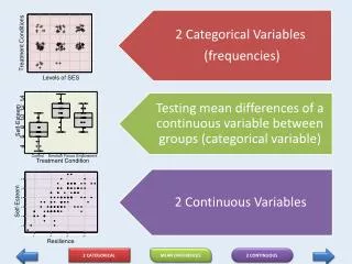
2. Categorical Variables • The raw data from categorical variables consist of group or category names that don’t necessarily have any ordering • Ordinal variables can be thought of as categorical variables for which the categories have a natural ordering • Could define categories for age, income or years of education

3. Categorical Variables • A study of 479 children found that children who slept either with a nightlight or in a fully lit room before the age of two had a higher incidence of myopia (nearsightedness) later in childhood.

4. Categorical Variables • Row percents show that the 2 variables are related • Incidence of myopia when the amount of sleep-time light increases • We can’t conclude that sleeping with light causes myopia, but we can say that the 2 variables are associated

5. Categorical Variables • To analyze relationship between 2 categorical variables • Calculate the percents within either the rows or the columns of the table • percents, like in the myopia table, are the percents across a row of a contingency table • percents are the percents down a column of a contingency table and are based on the total number of observations in the column

6. Categorical Variables • Sometimes, one variable can be designated as the variable and the other variable as the response variable. • In these situations it is customary to define the using the categories of the explanatory variable and the using the categories of the response variable

7. Categorical Variables

8. Categorical Variables • Need to calculate row percents to describe the relationship • Only interested in comparing divorce rates between smokers and nonsmokers • Of those who smoke • 49% (238/485) have been divorced • 51% (247/485) have not been divorced • Of those who don’t smoke • 32% (374/1184) have been divorced • 68% (810/1184) have not been divorced

9. Categorical Variables In a 1997 poll conducted by the Los Angeles Times, 1218 southern California residents were surveyed about their health and fitness habits. One of the questions was “What is the most important reason why you try to take care of your body: Is it mostly because you want to be attractive to others, or mostly because you want to keep healthy, or mostly because it helps your self-confidence, or what? Notice the pattern of responses is more or less the same for men and women. It seems reasonable to conclude that the response to the question was not related to the gender of the respondent.

10. Relative Risk • When a particular outcome is undesirable, researchers and journalists may describe the risk of that outcome • The that a randomly selected individual within a group falls into the undesirable category is simply the proportion in that category

11. Relative Risk • Common to express risk as a percent rather than a proportion • Suppose that within a group of 200 individuals, asthma affects 24 people • In this group the risk of asthma is = 0.12, or 12%

12. Relative Risk • Often want to know how the risk of an outcome relates to an explanatory variable • Use which is the ratio of the risks in two different categories of an explanatory variable

13. Relative Risk • Relative risk describes the risk in one group as a of the risk in another group • Suppose that a researcher states that, for those who drive while under the influence of alcohol, the relative risk of an automobile accident is 15 • The risk of an accident for those who drive under the influence is 15 times the risk for those who don’t drive under the influence

14. Relative Risk • Features of relative risk • When two risks are the same, the relative risk is • When two risks are different, the relative risk is different from • When the category in the numerator has higher risk, the relative risk is greater than 1 • The risk in the denominator (bottom) of the ratio is often the baseline risk, which is the risk for the category in which no additional treatment or behavior is present

15. Relative Risk • Refer back to the smoking and divorce example • To compute the relative risk of divorce for smokers, we first need to find the risk of divorce in each smoking category • For smokers, the risk of divorce is 238/485 = 0.491 or about • For nonsmokers, the risk of divorce is 374/1184 = 0.316 or about • This will be considered the be the risk of divorce

16. Relative Risk • Smoking and Divorce example, cont. • The relative Risk of divorce is the ratio of these two risks • In this sample, the risk of divorce for smokers is times the risk of divorce for nonsmokers

17. Percent Increase or Decrease in Risk • Sometimes an increase or decrease in risk is presented as a percent change instead of a multiple • The percent increase (or ) in risk can be calculated as follows:

18. Percent Increase or Decrease in Risk • Percent Increase in the Risk of Divorce for Smokers • We’ve already calculated the risk • Percent increase in risk = (1.53 - 1)*100% = • Get the same answer for the percent increase in risk by using the other formula:

19. Odds Ratio • Sometimes counts for the outcomes of a categorical variable are summarized by comparing the of one outcome to another, rather than by comparing one outcome to the total • The odds of getting a divorce to not getting a divorce for nonsmokers 374 divorced to 810 not divorced, or 0.46 divorced to 1 not divorced

20. Odds Ratio • For smokers, the odds are 238 divorced to 247 not divorced, of 0.96 to • Note these are approximately even odds • Odds are expressed using a phrase with the structure “ ” so a ratio is implied but not actually computed

21. Odds Ratio • The is used to compare the odds of a certain behavior or event within two different groups • May want to compare the odds of success versus failure for two different treatments of clinical depression • The odds ratio comparing the odds of divorce for smokers and nonsmokers is

22. Odds Ratio • The value of an odds ratio stays the same if the roles of the response and explanatory variables are • If we compared the odds of being a smoker for those who have divorced and those who haven’t the odds ratio is:

23. Summary

24. Confounding Variables • A variable is a variable that both affects the response variable and also is related to the explanatory variable. The effect of a confounding variable on the response variable cannot be separated from the effect of the explanatory variable • The term variable is sometimes used to describe a potential confounding variable that is not measured and is not considered in the interpretation of a study

25. Confounding Variables

26. Confounding Variables

27. Confounding Variables • When we look at the relationship between (the response variable) and (the explanatory variable) for each type of book separately, we see that the price does tend to increase with number of pages, especially for the technical books • Type of book (confounding variable) price (response variable) and type of book (confounding variable) number of pages (explanatory variable), because hardcover technical books tend to have fewer pages than paperback novels

28. Simpson’s Paradox • Occasionally, the effect of a confounding factor is strong enough to produce a paradox known as Simpson’s Paradox • The paradox is that the relationship appears to be in a direction when the confounding variable is not considered than when the data are separated into the categories of the confounding variable

29. Simpson’s Paradox • The following hypothetical data are similar to data from several actual studies looking at the association between oral contraceptive use and blood pressure

30. Simpson’s Paradox