Landscape Analysis and Animal Movement Analysis
460 likes | 1.01k Vues
Landscape Analysis and Animal Movement Analysis. RESM 575 Spring 2010 Lecture 14. Today. Part A Landscape analysis and metrics Part B Animal movement analysis. Putting landscape biodiversity in perspective.

Landscape Analysis and Animal Movement Analysis
E N D
Presentation Transcript
Landscape Analysis and Animal Movement Analysis RESM 575 Spring 2010 Lecture 14
Today Part A • Landscape analysis and metrics Part B • Animal movement analysis
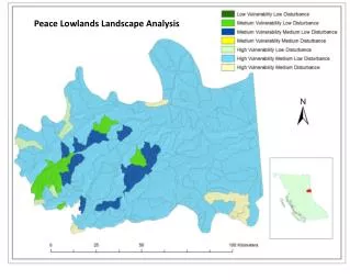
Putting landscape biodiversity in perspective Stein et al., 2006. Precious Heritage: The Status of Biodiversity in the United States. The Nature Conservancy.
Landscape (ecologist, env scientist) • a conceptual unit for the study of spatial patterns in the physical environment and the influence of these patterns on important environmental resources.
Landscape metrics • Goal is to study the pattern–process relationships • This has resulted in the development of literally hundreds of indices of landscape patterns. Ecological processes Spatial pattern
Landscape context • Landscapes don’t exist in isolation • They are nested within larger landscapes • Degree of “openness of a system” EX: from a geomorphological perspective, a watershed is a closed system EX: for a bird population, a watershed is an open system
Landscape scale • Most important consideration in an ecological landscape investigation • Must be explicitly defined • Describe patterns or relationships relative to scale • Be extremely cautious when attempting to compare landscapes measured at different scales
Classes of landscape pattern Applied to four types of spatial data: • Spatial point patterns • Linear network patterns • Surface patterns • Categorical map patterns
Spatial point patterns • The locations of the points are of primary interest rather than any quantity or quality • Clustered, random, dispersed?
Linear network patterns • Map of streams or riparian areas and the goal is to characterize the physical structure • Corridor density, connectivity, etc.
Surface patterns • No explicit boundaries, patches are not delineated, looking for spatial dependencies • Elevation, precipitation, continuous data
Categorical map patterns • Mosaic of discrete patches, land cover and use • Goal is to characterize the composition and spatial configuration • Most popular and the one we will focus on
Categorical map patterns • Characterization falls under: • Composition • Features associated with the variety and abundance of patch types but not considering the placement, attributes, or location of the patches in the mosaic • Spatial Configuration • refers to the spatial character and arrangement, position, or orientation of patches within the class or landscape.
Composition example metrics • Proportional abundance of each-class. • One of the simplest and perhaps most useful pieces of information that can be derived is the proportion of each class relative to the entire map. • Richness. • Simply the number of different patch types. • Eveness • The relative abundance of different patch types, typically emphasizing either relative dominance or its complement, equitability. • Diversity • Diversity is a composite measure of richness and evenness and can be computed in a variety of forms (e.g. Shannon’s, Simpson’s), depending on the relative emphasis placed on these two components
Spatial configuration example metrics • Characterization falls under • Patch size distribution and density • Mean, median, max, variance • Patch shape complexity • Simple and compact or irregular and convoluted, perimeter per area unit • Core areas • Interior area of patches, integrates patch size, shape, and edge effect distance into a single measure. • All other things being equal, smaller patches with greater shape complexity have less core area.
MORE! Spatial configuration example metrics • Characterization falls under • Isolation, proximity • Contrast • Dispersion • Contagion • Subdivision • Connectivity See link to McGarigal (1999) on website for more info
What makes a landscape metric useful? • A strong relationship between metric and functional response • The metric must pick up changes in the landscape that are important to a species or ecological process • EX:The black bear requires large intact forest patches of 125 acres or greater where does this habitat currently exist or where is that threshold of 125 acres being approached?
GIS role in measuring landscapes • Most GISs can calculate the basic metrics • All of the more sophisticated metrics use GIS data as inputs • FRAGSTATS http://www.umass.edu/landeco/research/fragstats/fragstats.html • ATILLA Analytical Tools Interface for Landscape Assessments http://www.epa.gov/nerlesd1/land-sci/attila/ • PATCH ANALYST http://flash.lakeheadu.ca/~rrempel/patch/
Limitations • Metrics are a snapshot in time • High degree of correlation among metrics (patch size, area, core area, edge, etc)
McGarigal (1999) suggests… Before selecting a metric: 1. Does it represent landscape composition or configuration, or both? 2. What aspect of composition or configuration does it represent? 3. Is it spatially explicit and, if so, at the patch-, class-, or landscape-level? 4. How is it affected by the designation of a matrix element? 5. Does it reflect an island biogeographical or landscape mosaic perspective of landscape pattern? 6. How does it behave or respond to variation in landscape pattern? 7. What is the range of variation in the metric under an appropriate spatiotemporal reference framework?
Typical landscape metrics • Fragmentation • Edge • Core area or interior forest
References • Boyce, M.S., and A. Haney. 1997. Ecosystem Management: Applications for Sustainable Forest and Wildlife Resources. Yale University Press, New Haven & London. 361 pages • Forman, R.T. T., and M. Godron. 1986. Landscape Ecology. Wiley, New York. • Grumbine, R. E. 1994. What is Ecosystem Management. Conservation Biology8:27-38. • Hobbs, R. 1997. Future Landscapes and the Future of Landscape Ecology. Landscape and Urban Planning 37:1-9. • Jones, B.K, K.H. Ritters, J. D. Wickham, R.D. Tankersley, R.V. ONeill, D.J. Chaloud, E. R. Smith, and A.C. Neale. 1997 An Ecological Assessment of United States Mid-Atlantic Region: A Landscape Atlas. • Benedic, M. A. and E. T. McMahon. 2000. Green infrastructure: smart conservation for the 21st century. The Sprawl Watch Clearinghouse Monograph Series, The Conservation Fund. • Grayson, R. B., I. D. Moore, and T. A. McMahon. 1992. Physically based hydrologic modeling: 1. A terrain based model for investigative purposes. Water Resources Research 28(10):2639-2658. • Loehle, C. 1999. Optimizing wildlife habitat mitigation with a habitat defragmentation algorithm. Forest Ecology and Management 120 (1999) 245-251 • Mitasova, H. J. Hofieka, M., Zlocha, L. R. Iverson. 1996. Modeling topographic potential for erosion and deposition using GIS. International Journal of Geographic Information Systems 10:629-641. • Riters, K. H. 1995. A Factor Analysis of Landscape Pattern and Structure Metrics. Landscape Ecology 10:23-39. • Wickham, J. D. Jones, K. B. Ritters, K. H. O’Neill, R. V. Tankersley, R. D. Smith, E. R. Neale, A. C. and Chaloud, D. J. 1999. An integrated environmental assessment of the US Mid-Atlantic Region. Environ Manag 24: 553-560. • Wickham, J. D., R. V. O’Neill, and K. B. Jones. 2000. Forest fragmentation as an economic indicator. Landscape Ecology 15: 171-179. • Wiens, J. 1976. 1976. Population responses to patchy environments. Ann. Rev. Ecol Syst. 7:81-120
Overview • Background on animal movement • Hawth’s tools
Field studies of animals • Commonly record the locations where individuals are observed. • In many cases these point data, often referred to as "fixes", are determined by radio telemetry. • These data may be used in both "basic" and "applied" contexts.
Using the point data or “fixes” • Used to test basic hypotheses • animal behavior • resource use • population distribution • interactions among individuals and populations.
Other uses of the point data • Location data may also be used in conservation and management of species. • The problem for researchers is • To determine which data points are relevant to their needs • How to best summarize the information.
Researchers using the point data • Rarely interested in every point that is visited, or the entire area used by an animal during its lifetime. • Focus on the animal's "home range“ • "…that area traversed by the individual in its normal activities of food gathering, mating, and caring for young. (Rogers and Carr, 1998)
Home range notes • Occasional sallies outside the area, perhaps exploratory in nature, should not be considered as in part of the “home range." (Burt 1943). • Thus, in its simplest form, "home range analysis" involves the delineation of the area in which an animal conducts its "normal" activities.
To maintain scientific integrity (repeatability) • Objective criteria must be used to select movements that are "normal" (White and Garrott 1990). • The obvious difficulty is in the definition of what should be considered "normal". • Because of this difficulty, there has been a proliferation of home range analysis models.
Home range models • Minimum convex polygons • Bivariate normal models • Jennrich-Turner estimator • weighted bivariate normal estimator, • multiple ellipses, • Dunn estimator • Nonparametric models • grid cell counts, • Fourier series smoothing, • harmonic mean • Contouring models • peeled polygons, • kernel methods, • hierarchical incremental cluster analysis
Of note: • However, home range analysis may involve more than just estimating the characteristics of areas occupied by animals. • Researchers often want to know about the distances, headings, times and speed of animal movements between locations. • They may also want to assess interactions of animals based on areas of overlap among home ranges or distances between individuals at a particular point in time. Most of these methods and their limitations have been reviewed by Harris et al. (1990) and White and Garrott (1990).
Hawth’s tools • Includes 2 home range analysis models: • minimum convex polygons (MCPs) and • kernel methods.
Minimum convex polygons • MCPs do not indicate how intensively different parts of an animal's range are used • Constructed by connecting the peripheral points of a group of points, such that external angles are greater than 180° (Mohr 1947). • "Percent" minimum convex polygons • "probability polygons" (Kenward 1987), • "restricted polygons" (Harris et al. 1990) • "mononuclear peeled polygons"
Kernal methods • Allow determination of centers of activity • Kernel analysis is a nonparametric statistical method for estimating probability densities from a set of points. • In the context of home range analysis these methods describe the probability of finding an animal in any one place. • Home range estimates are derived by drawing contour lines (i.e., isopleths) based on the volume of the curve under the utilization distribution. • Alternatively, isopleths can be drawn that connect regions of equal kernel density. In either case, the isopleths define home range polygons whose areas can be calculated.
References Burt, W. H. 1943. Territoriality and home range concepts as applied to mammals. J. Mammal. 24:346-352. (Harris, S., W. J. Cresswell, P. G. Forde, W. J. Trewhella, T. Woollard, and S. Wray 1990. Home-range analysis using radio-tracking data - a review of problems and techniques particularly as applied to the study of mammals. MammalRev. 20:97-123. Jones, M. C., J. S. Marron, and S. J. Sheather. 1996. A brief survey of bandwidth selection for density estimation. J. Amer. Stat. Assoc. 91:401-407. Kenward, R. 1987. Wildlife radio tagging. Academic Press, Inc., London, UK. 222 pp. Kenward, R. E., and K. H. Hodder. 1996. RANGES V: an analysis system for biological location data. Inst. Terrestrial Ecol., Furzebrook Res. Stn., Wareham, UK. 66 pp. Larkin, R. P., and D. Halkin. 1994. A review of software packages for estimating animal home ranges. Wildl. Soc. Bull. 22:274-287. Lawson, E. J. G., and A. R. Rodgers. 1997. Differences in home-range size computed in commonly used software programs. Wildl. Soc. Bull. 25:721-729. Michener, G. R. 1979. Spatial relationships and social organization of adult Richardson's ground squirrels. Can. J. Zool. 57:125-139.. Rodgers, A. R., R. S. Rempel, and K. F. Abraham. 1996. A GPS-based telemetry system. Wildl. Soc. Bull. 24:559-566. Schoener, T. W. 1981. An empirically based estimate of home range. Theor. Pop. Biol. 20:281-325. Seaman, D. E., and R. A. Powell. 1996. An evaluation of the accuracy of kernel density estimators for home range analysis. Ecology 77:2075-2085. Swihart, R. K., and N. A. Slade. 1985a. Testing for independence of observations in animal movements. Ecology 66:1176-1184. Swihart, R. K., and N. A. Slade. 1985b. Influence of sampling interval on estimates of home-range size. J. Wildl. Manage. 49:1019-1025. Worton, B. J. 1989. Kernel methods for estimating the utilization distribution in home-range studies. Ecology 70:164-168. Worton, B. J. 1995. Using Monte Carlo simulation to evaluate kernel-based home range estimators. J. Wildl. Manage. 59:794-800.