Download
1 / 37
370 likes | 400 Vues
Clustering Linear and Nonlinear Manifolds using Generalized Principal Components Analysis. René Vidal Center for Imaging Science Institute for Computational Medicine Johns Hopkins University. Data segmentation and clustering. Given a set of points, separate them into multiple groups

E N D
Clustering Linear and Nonlinear Manifolds using Generalized Principal Components Analysis René Vidal Center for Imaging Science Institute for Computational Medicine Johns Hopkins University
Data segmentation and clustering • Given a set of points, separate them into multiple groups • Discriminative methods: learn boundary • Generative methods: learn mixture model, using, e.g. Expectation Maximization
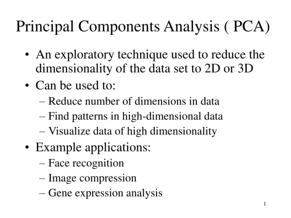
Dimensionality reduction and clustering • In many problems data is high-dimensional: can reduce dimensionality using, e.g. Principal Component Analysis • Image compression • Recognition • Faces (Eigenfaces) • Image segmentation • Intensity (black-white) • Texture
Clustering data on non Euclidean spaces • Clustering data on non Euclidean spaces • Mixtures of linear spaces • Mixtures of algebraic varieties • Mixtures of Lie groups • “Chicken-and-egg” problems • Given segmentation, estimate models • Given models, segment the data • Initialization? • Need to combine • Algebra/geometry, dynamics and statistics
Principal Component Analysis (PCA) • Given a set of points x1, x2, …, xN • Geometric PCA: find a subspace S passing through them • Statistical PCA: find projection directions that maximize the variance • Solution (Beltrami’1873, Jordan’1874, Hotelling’33, Eckart-Householder-Young’36) • Applications: data compression, regression, computer vision (eigenfaces), pattern recognition, genomics Basis for S
Generalized Principal Component Analysis • Given a set of points lying in multiple subspaces, identify • The number of subspaces and their dimensions • A basis for each subspace • The segmentation of the data points • “Chicken-and-egg” problem • Given segmentation, estimate subspaces • Given subspaces, segment the data
Basic ideas behind GPCA • Towards an analytic solution to subspace clustering • Can we estimate ALL models simultaneously using ALL data? • When can we do so analytically? In closed form? • Is there a formula for the number of models? • Will consider the most general case • Subspaces of unknown and possibly different dimensions • Subspaces may intersect arbitrarily (not only at the origin) • GPCA is an algebraic geometric approach to data segmentation • Number of subspaces = degree of a polynomial • Subspace basis = derivatives of a polynomial • Subspace clustering is algebraically equivalent to • Polynomial fitting • Polynomial differentiation
Introductory example: algebraic clustering in 1D Number of groups?
Introductory example: algebraic clustering in 1D How to compute n, c, b’s? Number of clusters Cluster centers Solution is unique if Solution is closed form if
Introductory example: algebraic clustering in 2D • What about dimension 2? • What about higher dimensions? • Complex numbers in higher dimensions? • How to find roots of a polynomial of quaternions? • Instead • Project data onto one or two dimensional space • Apply same algorithm to projected data
Representing one subspace • One plane • One line • One subspace can be represented with • Set of linear equations • Set of polynomials of degree 1
Representing n subspaces • Two planes • One plane and one line • Plane: • Line: • A union of n subspaces can be represented with a set of homogeneous polynomials of degree n De Morgan’s rule
Fitting polynomials to data points Veronese map • Polynomials can be written linearly in terms of the vector of coefficients by using polynomial embedding • Coefficients of the polynomials can be computed from nullspace of embedded data • Solve using least squares • N = #data points
Finding a basis for each subspace • To learn a mixture of subspaces we just need one positive example per class Polynomial Differentiation (GPCA-PDA) [CVPR’04]
Choosing one point per subspace • With noise and outliers • Polynomials may not be a perfect union of subspaces • Normals can estimated correctly by choosing points optimally • Distance to closest subspace without knowing segmentation?
GPCA for hyperplane segmentation • Coefficients of the polynomial can be computed from null space of embedded data matrix • Solve using least squares • N = #data points • Number of subspaces can be computed from the rank of embedded data matrix • Normal to the subspaces can be computed from the derivatives of the polynomial
Motion segmentation using GPCA • Apply polynomial embedding to 5-D points Veronese map
Experimental results: Kanatani sequences • Sequence A Sequence B Sequence C • Percentage of correct classification
Segmenting non-moving dynamic textures water A + z z v = 1 + t t t steam C + y z w = t t t • One dynamic texture lives in the observability subspace • Multiple textures live in multiple subspaces • Cluster the data using GPCA
Segmenting moving dynamic textures Ocean-bird
Temporal video segmentation Segmenting N=30 frames of a sequence containing n=3 scenes Host Guest Both Image intensities are output of linear system Apply GPCA to fit n=3 observability subspaces A + x x v = 1 + t t t C + dynamics y x w = t t t images appearance
Temporal video segmentation Segmenting N=60 frames of a sequence containing n=3 scenes Burning wheel Burnt car with people Burning car Image intensities are output of linear system Apply GPCA to fit n=3 observability subspaces A + x x v = 1 + t t t C + dynamics y x w = t t t images appearance
Overview of our approach • Propose a novel framework for simultaneous dimensionality reduction and clustering of data lying in different submanifolds of a Riemannian space. • Extend nonlinear dimensionality reduction techniques from one submanifold of to m submanifolds of a Riemannian space. • Show that when the different submanifolds are separated, all the points from one connected submanifold can be mapped to a single point in a low-dimensional space.
Nonlinear Dimensionality Reduction • Two kinds of dimensionality reduction: global and local techniques. • Global techniques • preserve global properties of the data lying on a submanifold • similar to PCA for a linear subspace • Eg: ISOMAP and Kernel PCA • Local techniques • preserve local properties, obtained from the small neighborhoods around the datapoints. • also retain the global properties of the data • Eg: Locally Linear Embedding (LLE), Laplacian Eigenmaps, Hessian LLE
Local Nonlinear Dimensionality Reduction • We show that segmentation of the data can be obtained from the null space of a matrix built from the local representation, using local NDR. • When the different submanifolds are separated, • there is a mapping from all the points in one connected submanifold to a single point in the low-dimensional space. • effectively reduces to a standard central clustering problem. • We will illustrate using Locally Linear Embedding (LLE).
Local Nonlinear Dimensionality Reduction • Focus on local NDR methods. Each method operates in a similar manner as follows: • Step 1: Find the k-nearest neighbors of each data point according to the Euclidean distance • Step 2: Compute a matrix , that depends on the weights . represents the local geometry of the data points and incorporates reconstruction cost function in low dimension. • Step 3: Solve a sparse eigenvalue problem on matrix . The first eigenvector is the constant vector corresponding to eigenvalue 0.
Extending LLE to Riemannian Manifolds • Information about the local geometry of the manifold is essential only in the first two steps of each algorithm, modifications are made only to these two stages. • Key issues: • how to select the kNN • by incorporating the Riemannian distance • how to compute the matrix representing the local geometry using the new metric.
Extending LLE to Riemannian Manifolds • LLE involves writing each data point as a linear combination of its neighbors. • Euclidean case, simply a least-squares problem • Riemannian case: one needs to solve an interpolation problem on the manifold. • How should the data points be interpolated? • What cost function should be minimized?
Clustering on Riemannian Manifolds • If the data lie in a disconnected union of k-connected submanifolds, the matrix is block-diagonal with blocks. • When the assumption of separated submanifolds is violated, we have and , respectively. • Hence, we can cluster the data into groups by applying k-means to the columns of a matrix whose rows are the eigenvectors in the null space of .
Motion Segmentation (SPSD(3) space) For Lambertian surfaces, spatial-temporal structure tensor
Segmenting fiber bundles in DTI (SPSD(3) space) • In DTI, the diffusion at each voxel is represented by a covariance matrix Cingulum Corpus Callosum Segmentation gives the separation between the two bundles. Corpus callosum: the red tensors pointing out of the plane and resembles the letter ‘C’. Cingulum: left to the corpus callosum with the green tensors oriented vertically.
Clustering of Probability Density Functions (Hilbert Unit Sphere) • Under square-root representation, the space of functions • Unit sphere, geometry is well-known
For more information, Vision, Dynamics and Learning Lab @ Johns Hopkins University Thank You!