2D/3D Shape Manipulation , 3D Printing
2D/3D Shape Manipulation , 3D Printing. Surface Reconstruction. Slides from Olga Sorkine. Geometry Acquisition Pipeline. Scanning: results in range images. Registration: bring all range images to one coordinate system. Stitching / reconstruction: Integration of scans into a single mesh.

2D/3D Shape Manipulation , 3D Printing
E N D
Presentation Transcript
2D/3D Shape Manipulation,3D Printing Surface Reconstruction Slides from Olga Sorkine
Geometry Acquisition Pipeline Scanning: results in range images Registration: bring all range images to one coordinate system Stitching/reconstruction: Integration of scans into a single mesh • Postprocess: • Topological and geometric filtering • Remeshing • Compression Olga Sorkine-Hornung
Digital Michelangelo Project 1G sample points → 8M triangles 4G sample points → 8M triangles Olga Sorkine-Hornung
Registration • Iterative Closest Points (ICP):Efficient Variants of the ICP Algorithm Connelly Barnes
reconstructed model set of raw scans Input to Reconstruction Process • Input option 1: just a set of 3D points, irregularly spaced • Need to estimate normals next class • Input option 2: normals come from the range scans Olga Sorkine-Hornung
How to Connect the Dots? • Explicit reconstruction: stitch the range scans together Olga Sorkine-Hornung
How to Connect the Dots? • Explicit reconstruction: stitch the range scans together • Connect sample points by triangles • Exact interpolation of sample points • Bad for noisy or misaligned data • Can lead to holes or non-manifold situations Olga Sorkine-Hornung
How to Connect the Dots? • Implicit reconstruction: estimate a signed distance function (SDF); extract 0-level set mesh using Marching Cubes Olga Sorkine-Hornung
How to Connect the Dots? • Implicit reconstruction: estimate a signed distance function (SDF); extract 0-level set mesh using Marching Cubes Olga Sorkine-Hornung
How to Connect the Dots? • Implicit reconstruction: estimate a signed distance function (SDF); extract 0-level set mesh using Marching Cubes • Approximation of input points • Watertight manifold results by construction Olga Sorkine-Hornung
How to Connect the Dots? • Implicit reconstruction: estimate a signed distance function (SDF); extract 0-level set mesh using Marching Cubes • Approximation of input points • Watertight manifold results by construction 0 < 0 > 0 Olga Sorkine-Hornung
Implicit vs. Explicit Input Implicit Explicit Olga Sorkine-Hornung
SDF from Points and Normals • Compute signed distance to the tangent plane of the closest point • Normals help to distinguish between inside and outside Olga Sorkine-Hornung + -
SDF from Points and Normals • Compute signed distance to the tangent plane of the closest point • Problem?? Olga Sorkine-Hornung
SDF from Points and Normals • Compute signed distance to the tangent plane of the closest point • The function will be discontinuous Olga Sorkine-Hornung
Smooth SDF • Instead find a smooth formulation for F. • Scattered data interpolation: • F is smooth • Avoid trivial 0 0 0 0 Olga Sorkine-Hornung
Smooth SDF • Scattered data interpolation: • F is smooth • Avoid trivial • Add off-surface constraints 0 0 0 0 Olga Sorkine-Hornung
Radial Basis Function Interpolation • RBF: Weighted sum of shifted, smooth kernels Smooth kernels (basis functions)centered at constrained points. For example: Scalar weights Unknowns Olga Sorkine-Hornung
Radial Basis Function Interpolation • Interpolate the constraints: 0 0 0 0 Olga Sorkine-Hornung
Radial Basis Function Interpolation • Interpolate the constraints: • Symmetric linear system to get the weights: Olga Sorkine-Hornung
RBF Kernels • Triharmonic: • Globally supported • Leads to dense symmetric linear system • C2smoothness • Works well for highly irregular sampling Olga Sorkine-Hornung
RBF Kernels • Polyharmonicspline • Multiquadratic • Gaussian • B-Spline (compact support) Olga Sorkine-Hornung
RBF Reconstruction Examples Olga Sorkine-Hornung
Off-Surface Points Properly chosen off-surface points Insufficient number/badly placed off-surface points Olga Sorkine-Hornung
Comparison of the various SDFs so far Distance to plane Compact RBF Global RBF Triharmonic Olga Sorkine-Hornung
RBF – Discussion • Global definition! • Global optimization of the weights, even if the basis functions are local 0 0 0 0 Olga Sorkine-Hornung
Extracting the Surface • Wish to compute a manifold mesh of the level set F(x) = 0 surface F(x) < 0 inside Image from: www.farfieldtechnology.com F(x) > 0 outside Olga Sorkine-Hornung
Sample the SDF Olga Sorkine-Hornung
Sample the SDF Olga Sorkine-Hornung
Tessellation • Want to approximate an implicit surface with a mesh • Can‘t explicitly compute all the roots • Sampling thelevelsetishard (rootfinding) • Solution: find approximate roots by trapping the implicit surface in a grid (lattice) + - - - Olga Sorkine-Hornung
Marching Squares • 16 different configurations in 2D • 4 equivalence classes (up to rotational and reflection symmetry + complement) … … Olga Sorkine-Hornung
Tessellation in 2D • 4 equivalence classes (up to rotational and reflection symmetry + complement) ? Olga Sorkine-Hornung
Tessellation in 2D • Case 4 is ambiguious: • Always pick consistently to avoid problems with the resulting mesh Olga Sorkine-Hornung
3D: Marching Cubes Layer k+1 Layer k Olga Sorkine-Hornung
Marching Cubes • Marching Cubes (Lorensen and Cline 1987) • Load 4 layers of the grid into memory • Create a cube whose vertices lie on the two middle layers • Classify the vertices of the cube according to theimplicit function (inside, outside or on the surface) Layer k+1 Layer k Olga Sorkine-Hornung
Marching Cubes • Compute case index. We have 28= 256 cases (0/1 for each of the eight vertices) – can store as 8 bit (1 byte) index. v8 v7 e7 e8 e6 v5 v6 e5 e6 e12 v6 e5 e11 e10 e9 v4 v3 e3 e10 e9 e4 e2 v1 v2 e1 e4 v1 e1 v1 v3 v4 v5 v6 v7 v8 v2 index = index = = 33 0 0 1 0 0 0 0 1 Olga Sorkine-Hornung
Marching Cubes • Unique cases (by rotation, reflection and complement) Olga Sorkine-Hornung
Tessellation3D – Marching Cubes • Using the case index, retrieve the connectivity in the look-up table • Example: the entry for index 33 in the look-up table indicates that the cut edges are e1; e4; e5; e6; e9 and e10 ; the output triangles are (e1; e9; e4) and (e5; e10; e6). e6 v6 e5 e10 e9 index = = 33 0 0 1 0 0 0 0 1 e4 v1 e1 Olga Sorkine-Hornung
Marching Cubes • Compute the position of the cut vertices by linear interpolation: • Move to the next cube
Marching Cubes – Problems • Haveto make consistent choices for neighboringcubes – otherwisegetholes – 3 3 Olga Sorkine-Hornung
Marching Cubes – Problems • Resolvingambiguities No Ambiguity Ambiguity Olga Sorkine-Hornung
Resolving Ambiguities • Marching Cubes 33 Connelly Barnes
Resolving Ambiguities Connelly Barnes
Resolving Ambiguities Connelly Barnes
Marching Cubes 33 Connelly Barnes
Marching Cubes 33 Connelly Barnes
Libraries • Short, portable code: • Paul Bourke -- Marching Cubes / Marching Tetrahedrons • Part of larger libraries/programs: • OpenMesh • MeshLab Connelly Barnes
Marching Cubes – Problems • Grid not adaptive • Many polygons required to represent small features Images from: “Dual Marching Cubes: Primal Contouring of Dual Grids” by Schaeffer et al. Olga Sorkine-Hornung
Marching Cubes – Problems Olga Sorkine-Hornung
Marching Cubes – Problems • Problems with short triangle edges • When the surface intersects the cube close to a corner, the resulting tiny triangle doesn‘t contribute much area to the mesh • When the intersection is close to an edge of the cube, we get skinny triangles (bad aspect ratio) • Triangles with short edges waste resources but don‘t contribute to the surface mesh representation Olga Sorkine-Hornung