ECE527: Holography and Diffractive Optics
250 likes | 533 Vues
ECE527: Holography and Diffractive Optics. Laboratory Experience # 1 Transmission Type Holograms. Date: September 10 th , 2012. Lecturer: Dr. Raymond Kostuk Prepared by: Juan Manuel Russo Email: jmrusso@ece.arizona.edu.

ECE527: Holography and Diffractive Optics
E N D
Presentation Transcript
ECE527: Holography and Diffractive Optics Laboratory Experience # 1 Transmission Type Holograms Date: September 10th, 2012. Lecturer: Dr. Raymond Kostuk Prepared by: Juan Manuel Russo Email: jmrusso@ece.arizona.edu Brief quotations from this presentation are allowable without special permission, provided that accurate acknowledgment of source is made.
Objectives • Become familiar with: • Photopolymer properties • Basic holographic recording: • Holographic exposure parameters. • Holographic recording procedure. • Reconstruction process. • Evaluate the properties of transmission holograms.
Actual setup picture (On pneumatic-dampened table.)
Laser Shutter L1 PH Actual setup picture with overlaid diagram (On pneumatic-dampened table.) L2 Hologram Plane M2 θ = 30º BS Folding Mirror M1
Holographic Setup • Components: • HeNe Laser at 633nm (coherent source) • Shutter (to control exposure Time) • Pin hole (10um) and Microscope Objective (20x): (Spatial filtering) • f = 30 cm plano-convex lens (Beam collimation and expansion). • 50/50 beam splitter. (Dividing the beam into two arms) • Folding mirror (to make setup more compact) • Mirrors 1 and 2. (Incidence angle) • Rotation Stage and sample holder. • Sample • Absorber • Path length difference (ABD – ACD in diagram) should be less than the coherence length (3-20cm for our HeNes) for maximum visibility of the interference pattern. (see http://www.ece.arizona.edu/~ece527/Coh-1.pdf )
Sample: Bayer Bayfol 102 HX • Photosensitive layer: • Chemistry for photoinitiated polymerization • 16 um thick • E = (18, 25, 30) mJ/cm2 exposure at λ = (633, 533, 455) nm respectively. • Index 1.52 • Panchromatic: sensible to all V IS spectrum. Work in total darkness (no safe light) • Glass substrate • ~2mm thick. • Index = 1.50 • Absorber: • Index matching fluid (nfluid = 1.499 - 1.52) • Glass with black paint to minimize reflection
Irradiance (mW/cm2)Measurement and Calculation • The irradiance at the hologram plane must be measured: • Measure the irradiance of each beam atperpendicular overfilling the detector. • Use the incidence angle of each beam to calculate the irradiance at the hologram plane: • Are the two irradiance terms too dissimilar? See note below. Note: If the irradiance at the hologram plane of the beams are too different from each other (more than 1:2), adjust the most powerful beam using a filter or modifying the setup to equalize the beams at the hologram plane. Try to achieve a beam to beam irradiance ratio of 1:1.
Measuring Irradiance (mW/cm2) • Silicon/Current meter detector example: • Hamamatsu S1226-44BK: • Area Adet = 0.137 cm2 • Responsivity (R) of 0.36A/W at 633nm. • Sensitivity of the detector is calculated: • The irradiance of each beam is calculated using: • Thorlabs S120VC silicon detector with a PM100D digital meter outputs Irradiance in mW/cm2 directly (used in this lab)
Exposure Time calculation • Exposure time: for an exposure E = 2800 – 3000 uJ/cm2 calculate how long () the sample has to be exposed with the previously calculated irradiance. • Set the shutter controller to that value.
Exposure Time Typical Results • Beam Irradiance at perpendicular: • E1 = 0.18 mW/cm2 and E2 = 0.24mW/cm2 • Unslanted setup: • Angles: θ1 = -θ2 = 15º • Beam ratio: E1cos(θ1) : E2cos(θ2) = 1 : 1.33 • For E = 18 mJ/cm2τ = 44 secs. • Slanted setup: • Angles: θ1 = 0º and θ2 = 30º • Beam ratio: E1cos(θ1) : E2cos(θ2) = 1 : 1.16 • For E = 18 mJ/cm2, τ = 46 secs.
Stabilize the environment • Holographic recording is susceptible to the environment: • Try to keep the exposure time to a minimum(i.e. higher power laser) • Turn off HVAC and/or any device that causes drifts or air currents in the room. • Mount the setup in a vibration-isolated table. (i.e. legs on sand, tube of a tire, pneumatic isolation system). • Make sure the room is light tight. Film is panchromatic. • No walking, talking, screaming or heavy breathing, if possible don’t be in the room. • Work on the ground floor of the building or in a lower level (underground basement, use a building away from busy streets, airports, trains, etc.) • Have a delay on your shutter so the environment stabilizes before exposure. • Test your environment. • Setup a Michelson interferometer • Magnify fringes • See if fringes drift, disappear or vary in intensity. All are indication of an unstable environment.
IN TOTAL DARKNESS Prepare to work in total darkness • Your eyes will not “get used to it” if the room is completely dark. • Remember where everything is and keep amount of things to do to a minimum. • Use tactile clues (screws, trays, poles) to be able to orient yourself in the room. • Do a dry run and see how you perform.
IN TOTAL DARKNESS Expose • PLACE THE SAMPLE IN THE HOLDER: Make sure the photopolymer side is facing the setup like is shown in the diagram. • Make sure lights are OFF and take the sample out of the light-tight box handling it ONLY by the edges. • Secure the sample (the holder should have screws or clamps).
Processing • This polymer is self-processing (i.e. no wet process) as the polymerization process initiated by the bright areas of the interference pattern continues until all the monomer is consumed. • Curing: since the dark areas of the interference pattern have unexposed photoinitiator, incoherent white light exposure (i.e. sunlight) can be used to increase transparency.
Resulting Structure • Bright areas of the interference pattern photoinitiate polymerization • Polymerization continues after exposure forming long chains in the bright areas (density increase) • Due to density gradient the unused monomer diffuses from dark to the bright areas. • Photocuring (exposure to incoherent white light) increases transparency. Reference: Journal of Photopolymer Science and Technology, Vol. 22 Number 2(2009) pages 257-260.
Measurement Procedure • Multiple spots (4 or 5) at different exposure levels were made. • Some spots were under exposed and others over exposed. • Optimum exposure found on the spot with the maximum D.E. • Angular spectrum was plotted. • Measurements are done in the same construction setup, blocking ONE beam, leaving the other as the reconstruction beam.
Equations for Measurement Analysis • Diffraction Efficiency: responsitivity cancels out, can be done with the current measurements from the detector directly. To take into account the Fresnel reflection losses from the first surface, use the detector to measure the reflected beam. • The efficiency is re-measured for different incident angles and plotted vs. the deviation from the Bragg angle (equal or very close to the construction angle).
Results Diffraction Efficiency vs. Incident angle plot obtained from the reference cited below. Reference: Journal of Photopolymer Science and Technology, Vol. 22 Number 2(2009) pages 257-260.