Matrix Operations and Curve Fitting Analysis
Learn about matrix operations, Gaussian Elimination, and curve fitting analysis in this lecture. Understand the application of matrices in modeling and analyze data for curve fitting.

Matrix Operations and Curve Fitting Analysis
E N D
Presentation Transcript
Lecture 3Matrices Lat Time Matrices, Gaussian Elimination and Gauss-Jordan Elimination Operation with Matirces Properties of Matrix Operations Reading Assignment: Sec. 1.1 and 2.1of Text Elementary Linear Algebra R. Larsen et al. (5 Edition) TKUEE翁慶昌-NTUEE SCC_09_2007
Application: Model/Curve Fitting • Problem Description • A baseball analyst says that “Wang’s strike out rate (SO) is parabolic function of his average pitch speed (v)” • You are suspicious of the analyst’s theory. So you collect some data about Wang’s pitching performance as follows: • Now you want to find out if a parabolic function is a good model of SO = f(v)
Ideas • I1: Mathematical formulation of the analyst’s theory SO = f(v) = av2 + bv + c • I2: There are 6 data points but only three unknowns (a, b, and c)
Least Square Error Fit • I3: Now we define a good fit criteria: Least Square Error Square Error (SE) = J(a, b, c)
Least Error Fit from Linear Equations • I4: Least Square Error Fit by Solving dJ(a,b,c)/da = 0 (1) dJ(a,b,c)/db = 0 (2) dJ(a,b,c)/dc = 0 (3) Fact: to find min f(x), we solve df(x)/dx = 0 first. Let the solution be x*. If d2f(x*)/dx2 < 0, then x* is the minimum solution. • I5: Equations (1) – (3) are linear equations of a,b, and c.
Least Error Fit from Linear Equations • I6: By solving the three linear equations of a, b and c, we find a least square error fit SO = f(v) = av2 + bv + c to the data points. • The square error J(a,b,c) indicates how good the fit is to the 6 data points and we can check how good the analyst’s model is. • This LSE fit method is applicable to • any number of data points • Polynomial function f(.) of any order n and ends up solving a set of linear equations of n-variables (the n coefficients of the order-n polynomial function.
Lecture 3: Matrices Today • Properties of Matrix Operations • Inverse • Applications: Economics and Mgmt. and Engrg. Reading Assignment: Secs 2.2-2.5 of Textbook Homework #1 Due http://en.wikipedia.org/wiki/Determinant#Determinants_of_2-by-2_matrices Next Time • Elementary Matrices • Determinant of a Matrix • Evaluation of Determinant Reading Assignment: Secs 3.1-3.2 of Textbook
Lecture 3: Matrices Today • Properties of Matrix Operations • Inverse of a Matrix • Applications: Economics and Mgmt. and Engrg.
Keywords in Section 2.1: • row vector: 列向量 • column vector: 行向量 • diagonal matrix: 對角矩陣 • trace: 跡數 • equality of matrices: 相等矩陣 • matrix addition: 矩陣相加 • scalar multiplication: 純量積 • matrix multiplication: 矩陣相乘 • partitioned matrix: 分割矩陣
2.2 Properties of Matrix Operations • Three basic matrix operators: • (1) matrix addition • (2) scalar multiplication • (3) matrix multiplication • Zero matrix: • Identity matrix of order n:
Thm 2.1 Properties of matrix addition and scalar multiplication: Then (1) A+B = B + A (2) A + ( B + C ) = ( A + B ) + C (3) ( cd ) A = c ( dA ) (4) 1A = A (5) c( A+B ) = cA + cB (6) ( c+d ) A = cA + dA
Notes: • 0m×n: the additive identity for the set of all m×n matrices • –A: the additive inverse of A • Properties of zero matrices:
Properties of the identity matrix: • Properties of matrix multiplication: (1) A(BC) = (AB ) C (2) A(B+C) = AB + AC (3) (A+B)C = AC + BC (4) c (AB) = (cA) B = A (cB)
Sol: (a) (b) (c) • Ex: (Find the transpose of the following matrix) (a) (b) (c)
Ex: is symmetric, find a, b, c? Sol: Q: Will A stay symmetric by a row exchange? • Symmetric matrix: A square matrix A is symmetric if A = AT • Skew-symmetric matrix: A square matrix A is skew-symmetric if AT = –A
Note: is symmetric Pf: • Ex: is a skew-symmetric, find a, b, c? Sol:
Matrix: Three situations: • Real number: ab = ba (Commutative law for multiplication) (Sizes are not the same) (Sizes are the same, but matrices are not equal)
Note: • Ex 4: Sow that AB and BA are not equal for the matrices. and Sol:
Real number: (Cancellation law) • Matrix: (1) If C is invertible, then A = B (Cancellation is not valid)
Sol: So But • Ex 5:(An example in which cancellation is not valid) Show that AC=BC
Keywords in Section 2.2: • zero matrix: 零矩陣 • identity matrix: 單位矩陣 • transpose matrix: 轉置矩陣 • symmetric matrix: 對稱矩陣 • skew-symmetric matrix: 反對稱矩陣
2.3 The Inverse of a Matrix • Note: A matrix that does not have an inverse is called noninvertible (or singular). • Inverse matrix: Consider Then (1) A is invertible (or nonsingular) (2) B is the inverse of A
Pf: • Notes: (1) The inverse of A is denoted by • Thm 2.7: (The inverse of a matrix is unique) If B and C are both inverses of the matrix A, then B = C. Consequently, the inverse of a matrix is unique.
Sol: • Find the inverse of a matrix by Gauss-Jordan Elimination: • Ex 2: (Find the inverse of the matrix)
Note: If A can’t be row reduced to I, then A is singular.
Sol: • Ex 3: (Find the inverse of the following matrix)
Check: So the matrix A is invertible, and its inverse is
Thm 2.8:(Properties of inverse matrices) If A is an invertible matrix, k is a positive integer, and c is a scalar, then
Pf: • Note: • Thm 2.9: (The inverse of a product) • If A and B are invertible matrices of size n, then AB is invertible and
Thm 2.10 (Cancellation properties) • If C is an invertible matrix, then the following properties hold: • (1) If AC=BC, then A=B (Right cancellation property) • (2) If CA=CB, then A=B (Left cancellation property) Pf: • Note: IfC is not invertible, then cancellation is not valid.
Pf: ( A is nonsingular) • Thm 2.11: (Systems of equations with unique solutions) If A is an invertible matrix, then the system of linear equations Ax = b has a unique solution given by (Left cancellation property) This solution is unique.
Keywords in Section 2.3: • inverse matrix: 反矩陣 • invertible: 可逆 • nonsingular: 非奇異 • singular: 奇異 • power: 冪次
Applications • Model/Curve Fitting • Failure Prune Machine Capacity Modeling • Network Flow • Power Flow

![[MATRICES ]](https://cdn4.slideserve.com/144276/matrices-dt.jpg)