Solar and Stellar dynamos
960 likes | 981 Vues
This article explores the observations and basic theory of solar and stellar dynamos, including mean field electrodynamics and various mechanisms for producing a poloidal field. It also discusses the mathematical considerations of mean field models and presents robust results from global solar and stellar models. Additionally, it examines the solar cycle, sunspots, magnetic fields, and other related phenomena.

Solar and Stellar dynamos
E N D
Presentation Transcript
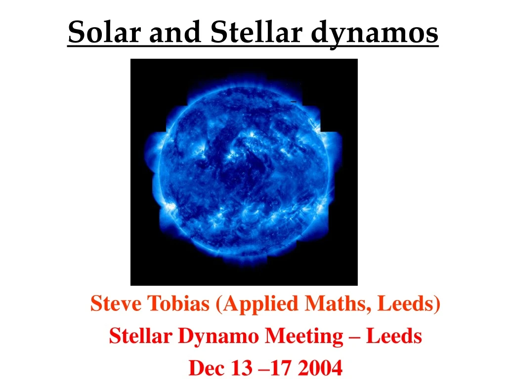
Solar and Stellar dynamos Steve Tobias (Applied Maths, Leeds) Stellar Dynamo Meeting – Leeds Dec 13 –17 2004
Observations Some basic theory Mean Field Electrodynamics The simplest solutions a-effect, a-quenching Big argument Other mechanisms for producing poloidal field What physics do we need to understand? Cartoon Pictures of solar dynamo a-effect Distributed Flux conveyor Interface Dynamos Talk Summary • Robust (general) results from mean field models • Mathematical considerations of the mean field equations • Low order models • Global Solar Dynamo Models • Specifically Stellar Models • See reviews by Ossendrijver (2003), Weiss & Tobias (2005)
Observations: Solar Magnetogram of solar surface shows radial component of the Sun’s magnetic field. Active regions: Sunspot pairs and sunspot groups. Strong magnetic fields seen in an equatorial band (within 30o of equator). Rotate with sun differentially. Each individual sunspot lives ~ 1 month. As “cycle progresses” appear closer to the equator.
Sunspots Dark spots on Sun (Galileo) cooler than surroundings ~3700K. Last for several days (large ones for weeks) Sites of strong magnetic field (~3000G) Axes of bipolar spots tilted by ~4 deg with respect to equator Arise in pairs with opposite Polarity Part of the solar cycle Fine structure in sunspot umbra and penumbra
Observations Solar (a bit of theory) Sunspot pairs are believed to be formed by the instability of a magnetic field generated deep within the Sun. Flux tube rises and breaks through the solar surface forming active regions. This instability is known as Magnetic Buoyancy. It is also important in Galaxies and Accretion Disks and Other Stars. Wissink et al (2000)
Observations: Solar BUTTERFLY DIAGRAM: last 130 years Migration of dynamo activity from mid-latitudes to equator Polarity of sunspots opposite in each hemisphere (Hale’s polarity law). Tend to arise in “active longitudes” DIPOLAR MAGNETIC FIELD Polarity of magnetic field reverses every 11 years. 22 year magnetic cycle.
Observations Solar • Solar cycle not just visible in sunspots • Solar corona also modified as cycle progresses. • Weak polar magnetic field has mainly one polarity at each pole and two poles have opposite polarities • Polar field reverses every 11 years – but out of phase with the sunspot field. • Global Magnetic field reversal.
Observations: Solar SUNSPOT NUMBER: last 400 years Maunder Minimum Modulation of basic cycle amplitude (some modulation of frequency) Gleissberg Cycle: ~80 year modulation MAUNDER MINIMUM: Very Few Spots , Lasted a few cycles Coincided with little Ice Age on Earth Abraham Hondius (1684)
Observations: Solar RIBES & NESME-RIBES (1994) BUTTERFLY DIAGRAM: as Sun emerged from minimum Sunspots only seen in Southern Hemisphere Asymmetry; Symmetry soon re-established. No Longer Dipolar? Hence: (Anti)-Symmetric modulation when field is STRONG Asymmetric modulation when field is weak
Observations: Solar - helicities • Important observational indices for dynamo theory are kinetic helicity , current helicity and magnetic helicity • can be estimated from vector magnetograms • At a given latitude, distribution about a mean value that is negative at in Northern Hemisphere • is not easy to measure • Suggestive that negative in NH (Berger & Ruzmaikin 2000) • Proxy of kinetic helicity can be measured (Duvall & Gizon 2000) and is negative in the NH
14 14 C C 10 10 Be Be Observations: Solar (Proxy) PROXY DATA OF SOLAR MAGNETIC ACTIVITY AVAILABLE SOLAR MAGNETIC FIELD MODULATES AMOUNT OF COSMIC RAYS REACHING EARTH responsible for production of terrestrial isotopes : stored in ice cores after 2 years in atmosphere : stored in tree rings after ~30 yrs in atmosphere BEER (2000)
Observations: Solar (Proxy) Cycle persists through Maunder Minimum (Beer et al 1998) DATA SHOWS RECURRENT GRAND MINIMA WITH A WELL DEFINED PERIOD OF ~ 208 YEARS Wagner et al (2001)
Solar Structure Solar Interior • Core • Radiative Interior • (Tachocline) • Convection Zone Visible Sun • Photosphere • Chromosphere • Transition Region • Corona • (Solar Wind)
The Large-Scale Solar Dynamo • Helioseismology shows the internal structure of the Sun. • Surface Differential Rotation is maintained throughout the Convection zone • Solid body rotation in the radiative interior • Thin matching zone of shear known as the tachocline at the base of the solar convection zone (just in the stable region).
Torsional Oscillations and Meridional Flows • In addition to mean differential rotation there are other large-scale flows • Torsional Oscillations • Pattern of alternating bands of slower and faster rotation • Period of 11 years (driven by Lorentz force) • Oscillations not confined to the surface (Vorontsov et al 2002) • Vary according to latitude and depth
Torsional Oscillations and Meridional Flows • Meridional Flows • Doppler measurements show typical meridional flows at surface polewards: velocity 10-20ms-1 (Hathaway 1996) • Poleward Flow maintained throughout the top half of the convection zone (Braun & Fan 1998) • No evidence of returning flow • Meridional flow at surface advects flux towards the poles and is probably responsible for reversing the surface polar flux
Observations: Stellar (Solar-Type Stars) Stellar Magnetic Activity can be inferred by amount of Chromospheric Ca H and K emission Mount Wilson Survey (see e.g. Baliunas ) Solar-Type Stars show a variety of activity. Cyclic, Aperiodic, Modulated, Grand Minima
Observations: Stellar (Solar-Type Stars) • Activity is a function of spectral type/rotation rate of star • As rotation increases: activity increases • modulation increases • Activity measured by the relative Ca II HK flux density • (Noyes et al 1994) • But filling factor of magnetic fields also changes • (Montesinos & Jordan 1993) • Cycle period • Detected in old slowly-rotating G-K stars. • 2 branches (I and A) (Brandenburg et al 1998) • WI ~ 6 WA (including Sun) Wcyc/Wrot ~ Ro-0.5(Saar & Brandenburg 1999)
LARGE SCALE Sunspots Butterfly Diagram 11-yr activity cycle Coronal Poloidal Field Systematic reversals Periodicities ------------------------------ Field generation on scales > LTURB SMALL SCALE Magnetic Carpet Field Associated with granular and supergranular convection Magnetic network --------------------------------- Field generation on scales ~ LTURB Large and Small-scale dynamos
Basics for the Sun Dynamics in the solar interior is governed by the following equations of MHD INDUCTION MOMENTUM CONTINUITY ENERGY GAS LAW
1020 1016 1013 1012 1010 106 10-7 10-7 105 1 10-3 10-6 10-4 1 0.1-1 10-3-0.4 BASE OF CZ Basics for the Sun PHOTOSPHERE (Ossendrijver 2003)
Modelling Approaches • Because of the extreme nature of the parameters in the Sun and other stars there is no obvious way to proceed. • Modelling has typically taken one of three forms • Mean Field Models (~85%) • Derive equations for the evolution of the mean magnetic field (and perhaps velocity field) by parametrising the effects of the small scale motions. • The role of the small-scales can be investigated by employing local computational models • Global Computations (~1%) • Solve the relevant equations on a massively-parallel machine. • Either accept that we are at the wrong parameter values or claim that parameters invoked are representative of their turbulent values. • Maybe employ some “sub-grid scale modelling” e.g. alpha models • Low-order models • Try to understand the basic properties of the equations with reference to simpler systems (cf Lorenz equations and weather prediction) • All 3 have strengths and weaknesses
Starting point is the magnetic induction equation of MHD: where B is the magnetic field, u is the fluid velocity and η is the magnetic diffusivity (assumed constant for simplicity). Assume scale separation between large- and small-scale field and flow: where B and U vary on some large length scale L, and u and b vary on a much smaller scale l. where averages are taken over some intermediate scale l « a « L. Kinematic Mean Field Theory
For simplicity, ignore large-scale flow, for the moment. Induction equation for mean field: where mean emf is This equation is exact, but is only useful if we can relate to Consider the induction equation for the fluctuating field: Where “pain in the neck term”
(and hence between and and Under this assumption, the relation between ) is linear and homogeneous. Traditional approach is to assume that the fluctuating field is driven solely by the large-scale magnetic field. i.e. in the absence of B0 the fluctuating field decays. i.e. No small-scale dynamo (not really appropriate for high Rm turbulent fluids)
α: regenerative term, responsible for large-scale dynamo action. Since is a polar vector whereas Bis an axial vector then α can be non-zero only for turbulence lacking reflexional symmetry (i.e. possessing handedness). β: turbulent diffusivity. Postulate an expansion of the form: where αij and βijk are pseudo-tensors, determined by the statistics of the turbulence. Simplest case is that of isotropic turbulence, for which αij = αδij and βijk = βεijk. Then mean induction equation becomes: BUT WHAT ARE a and b ? MORE LATER
BASIC PROPERTIES OF THE MEAN FIELD EQUATIONS Add backin the mean flow U0 and the mean field equation becomes Now consider simplest case where a = a0 cos q andU0 = U0 sin q ef In contrast to the induction equation, this can be solved for axisymmetric mean fields of the form
BASIC PROPERTIES OF THE MEAN FIELD EQUATIONS • Linear growth-rate of B0 depends on dimensionless combination of parameters. • Critical parameter given by • If |D| > Dc then exponentially growing solutions are found – dynamo action. • Estimates suggest |Da| ~ 2, |DW| ~ 103 for the Sun and hence one can make the aW-approximation where the a-effect is ignored in generating the toroidal field. • Can also have a2W and a2 dynamos – may be of relevance for fully convective or more rapidly rotating stars.
BASIC PROPERTIES OF THE MEAN FIELD EQUATIONS • In general B0 takes the form of an exponentially growing dynamo wave that propagates. • Direction of propagation depends on sign of dynamo number D. • If D > 0 waves propagate towards the poles, • If D < 0 waves propagate towards the equator. • In this linear regime the frequency of the magnetic cycle Wcyc is proportional to |D|1/2 • Solutions can be either dipolar or quadrupolar
Crucial questions Mean field electrodynamics therefore seems to work very well - but there are some very obvious questions to ask How can we calculate a and b? What will these be in the Sun. Can we relate them to the properties of the flow in the kinematic regime? 2. Even if we know how a and b behave kinematically, what is the role of the Lorentz force on the transport coefficients α and β? 3. How weak must the large-scale field be in order for it to be dynamically insignificant? Dependence on Rm?
1. How can we calculate a and b? Can we relate them to the properties of the flow in the kinematic regime? • Of course a and b can only really be calculated by determining • But we can only know bif we solve the fluctuating field equation. • Analytic progress can be made by making one of two approximations • Either Rm or the correlation time of the turbulence tcorr is small. • Then can ignore “pain in the neck” G term in fluctuating field equation. • Get famous results that a is related to the helicity of the flow with a constant of proportionality given by the small parameter e.g. • Note we have parameterised correlations between u and b by correlations between u and w
1. How can we calculate a and b? Can we relate them to the properties of the flow in the kinematic regime? • We could do some numerical experiments and simply measure a • The best way to do this is to impose a known mean field B and then calculate numerically • If the Lorentz force is switched off (the field is weak) then this gives a kinematic calculation of a. • Example: Choose a flow with Rm not small and not at short correlation time and simply evaluate a. • So we solve the kinematic induction equation With an applied mean field to calculate E. Here we choose u to be the famous G-P flow
1. How can we calculate a and b? Can we relate them to the properties of the flow in the kinematic regime? • For this flow the a term is a tensor. • The a-effect is a very sensitive function of Rm. • It even changes sign. • It can in no way be related in a simple manner to the helicity of the flow (bit of a strange flow as it has infinite correlation time) • Neither of the approximations work very well at high Rm • Changes in correlation times may change results… a g Rm Rm Courvoisier et al 2004
T0 Ω g T0 + ΔT Rotating turbulent convection (Cattaneo & Hughes 2005) Sometimes it is not even possible to calculate a turbulent a-effect Boussinesq convection. Taylor number, Ta = 4Ω2d4/ν2 = 5 x 10⁵, Ro = 1/10-1/5 Prandtl number Pr = ν/κ = 1, Magnetic Prandtl number Pm = ν/η = 5. Critical Rayleigh number = 59 008. Anti-symmetric helicity distribution anti-symmetric α-effect. Maximum relative helicity ~ 1/3.
Ra = 150 000 Weak imposed field in x-direction. Temperature on a horizontal slice close to the upper boundary. Ra = 150,000. No dynamo at this Rayleigh number – but still an α-effect. Mean field of unit magnitude imposed in x-direction (essentially kinematic) Self-consistent dynamo action sets in at Ra 200,000.
e.m.f. and time-average of e.m.f. Ra = 150,000 Imposed Bx = 1. Imposed field extremely weak – kinematic regime. time time time
Cumulative time average of the e.m.f. Not fantastic convergence. α – the ratio of e.m.f. to applied magnetic field – is very small. And even depends on Rm!!! Note this is not a-suppression (field too weak) It appears that the α-effect here is not turbulent (i.e. fast), but diffusive (i.e. slow). However in models of rotating compressible convection, Ossendrijver et al (2002) find a significant a-effect -- fewer cells in box? -- less turbulent? -- less incoherence (decoherence)?
Bx No evidence of significant energy in the large scales – either in the kinematic eigenfunction or in the subsequent nonlinear evolution. Picture entirely consistent with an extremely feeble α-effect. Note Jones & Roberts (2002) find a large mean field. As you go to bigger boxes and more cells it is harder to get a mean field or measure an a-effect
2. How are a and b modified by the mean field in the Nonlinear Regime? • This is a CRUCIAL question. • Assume kinematic theory is OK (hmm) • The mean field <B> will act back on the turbulence so as to switch off the generation mechanism via the Lorentz Force. • When does this happen? • Traditional argument… • This occurs when mean field reaches equipartition with the turbulence so
2. How are a and b modified by the mean field in the Nonlinear Regime? • But… • It is the small scale magnetic field that will act back on the small-scale turbulence. • The dynamo will switch off when the small-scale magnetic energy becomes comparable with the small-scale kinetic energy of the flow. • There are many different possibilities, but it seems clear that due to amplification by the turbulence the small scale magnetic field is much bigger than the mean magnetic field From a simple scaling it follows that: where p is a flow and geometry dependent coefficient (p>0)
2. How are a and b modified by the mean field in the Nonlinear Regime? • This poses a major problem for mean field theory (see Proctor 2003;Diamond et al 2004 for an erudite discussion) • If true then this implies that the a-effect (and probably the b-effect) is switched off when the mean magnetic field is small (i.e. when • Hence the source term (a) will be catastrophically quenched when the mean field is very small. • Is this correct? • Two ways of checking • Analytical results based on approximations • Numerical results at moderate Rm
2. How are a and b modified by the mean field in the Nonlinear Regime? ANALYTICAL RESULTS • Really again we have to solve the induction equation for b and the momentum equation for u to calculate a and b viaE • But some analytical progress is made by following two strands • Take some exact results • e.g. Integrated Ohm’s Law • Conservation of magnetic helicity due to small scales • General Conservation of magnetic helicity(e.g. Brandenburg & Dobler 2001)
2. How are a and b modified by the mean field in the Nonlinear Regime? ANALYTICAL RESULTS The second strand is to combine these exact results (or modifications thereof) with an approximate result for a in the nonlinear regime • Note: This is not an exact result. • It is derived using the EDQNM approximation • Only applies (if at all) for short correlation times and assumes that the magnetic field does not affect the correlation time of the turbulence. • Also have to be careful about the meanings of in this formula (Proctor 2003) Pouquet, Frisch & Léorat 1976
2. An aside – what do Pouquet, Frisch and Léorat actually do?(Proctor 2003) • They take a state of pre-existing helical MHD turbulence which is happily minding its own business with small scale b and u (but no large scale field?). • They add a weak mean field to this and linearise the equations to get equations for the perturbations to u and b (u’ and b’) • They make a short correlation time approximation to say that
2. How are a and b modified by the mean field in the Nonlinear Regime? ANALYTICAL RESULTS • By combining these two results (or similar) it is possible to get formulae for a (and b) • Gruzinov and Diamond 1994,1995, 1996 • Blackman & Field 2000, Blackman & Brandenburg 2002 • Kleeorin et al 1995 • And many more… • e.g.
2. How are a and b modified by the mean field in the Nonlinear Regime? NUMERICAL RESULTS • As in the kinematic regime can be calculated numerically and related to an applied mean field • This can be done for forced flows or for convection for various values of and Rm. • e.g. for Galloway-Proctor flow solve
Components of e.m.f. versus time.
α versus B02 (Cattaneo & Hughes 1996) Suggestive of the formula: for γ = O(1). α versus Rm (C, H & Thelen 2002)
Mean Field Hydrodynamics • Of course, mean field theory can be played on the Navier-Stokes equations (see e.g. Rüdiger 1989). • Solve equations for mean flow and parameterise small-scale interactions. • This is even more dodgy as there is no closure that relates the small scale flows to the mean velocity. • Also have to worry about Galilean Invariance of equations Reynolds Stress Mean Lorentz Force Maxwell Stress
Other Possible Mechanisms for Producing Poloidal Field • In addition to the conventional turbulent driven a-effect, there have been other mechanisms suggested for generating a large scale poloidal field • Most of these are dynamic and rely on the presence of a large-scale toroidal field.