Equilibrium Business-Cycle Model and Technology Shocks
180 likes | 215 Vues
Understand how technology shocks impact real GDP and macroeconomic variables in an equilibrium business-cycle model. Learn how Solow Residuals and empirical tests help measure technology shocks and predict changes in real wage, GDP, rental price of capital, interest rate, and consumption/investment equilibrium. Explore the implications and analysis of these predictions in the model.

Equilibrium Business-Cycle Model and Technology Shocks
E N D
Presentation Transcript
An Equilibrium Business-Cycle Model Mr. Vaughan Income and Employment Theory (402)
Lecture Outline • Source of Shocks – Equilibrium Model • Technology (A): Permanent vs. Temporary • Empirical Predictions of Equilibrium Model • Real Wage • Real Price of Capital Services • Interest Rate • Consumption and Investment
Equilibrium Business-Cycle Model • Uses equilibrium conditions to determine how shocks affect real GDP (Y) and other macroeconomic variables, such as consumption (C) and net investment (I). • Model: Real output determined by production function (prices adjust to insure consumption + net investment equals real output). • Y= A· F(K, L) • Capital stock (K)fixed in short run • Labor input (L) is fixed (by assumption) • Impulse mechanism: Technology shocks (i.e., changes in Yreflect only changes in technology, “A”). • Positive shock (A↑) implies boom (Y↑) • Negative shock (A↓) implies recession (Y↓)
How Are Technology Shocks Measured? Solow Growth Model in Action • Real Business Cycle (RBC) macroeconomists use Solow Residualsto identify technology shocks. Recall growth accounting equation: ∆Y/Y = ∆A/A + α·(∆K/K) + (1 - α )·(∆L/L) (3.4) • Rearranging yields: ∆A/A = ∆Y/Y – [α·(∆K/K) + (1 - α )·(∆L/L)] (3.22) • Level of technology (A) is not observable, so technology shocks (∆A/A) cannot be directly measured. But terms on right side of (3.22) can be quantified with national income account data. • RBC economists use Solow Residuals (∆A/A) to “shock” general-equilibrium models, then compare behavior of artificial with actual economy. • Result: Behavior of artificial economy looks remarkably like actual post-WWII U.S. economy. (By construction, time path of output in artificial economy is Pareto Optimal, so RBC’s reason, time path of U.S. economy must be as well).
Equilibrium Business-Cycle ModelEmpirical Tests Model Prediction: Real Wage (w/P) and Real GDP (Y)? • Advance in technology (A↑) raises real output (Y↑). • Advance in technology raises marginal product of labor, MPL, for given inputs of capital (K) and labor (L). Y= A·F(K,L) MPL = ∂Y/∂L = A·FL A↑ => MPL↑ • MPL curve is demand for labor curve, so increase in technology shifts demand to right (increase) • Real wage rises to clear labor market (w/P↑) • Result: Pro-cyclical real wage
Equilibrium Business-Cycle ModelEmpirical Tests • Analysis • Increase in A raises Y. • Increase in A raises w/P. • Implication: Pro-cyclical real wage • (squares with stylized facts)
Equilibrium Business-Cycle ModelEmpirical Tests Model Prediction: Real Rental Price of Capital and Real GDP? • Advance in technology (A↑) raises real output (Y↑). • Advance in technology raises marginal product of labor, MPK, for given inputs of capital (K) and labor (L). Y= A·F(K, L) MPK = ∂Y/∂K = A·Fk A↑ => MPK↑ • MPK curve is demand for capital curve, so increase in technology shifts demand to the right (increase). • Real rental price rises to clear capital market (R/P↑) • Prediction: Pro-cyclical real rental price of capital.
Equilibrium Business-Cycle ModelEmpirical Tests • Analysis • Increase in A raises Y. • Increase in A raises R/P. • Implication:Pro-cyclical real rental price (squares with stylized facts)
Equilibrium Business-Cycle ModelEmpirical Tests Model Prediction: Interest Rate and Real GDP? • Recall: • i = R/P − δ • i = MPK (evaluated at given K and L) − δ • δ is given. • Advance in technology (A↑)boosts real GDP (Y↑) • Advance in technology (A↑)boosts marginal product of capital (MPK↑), at given inputs of capital (K) and labor (L). • Interest rate (i↑) rises with MPK (MPK↑) • Prediction: Interest rate is pro-cyclical. • Model predicts an economic boom will produce a relatively high interest rate, whereas a recession will produce produces a relatively low interest rate.) • Squares with stylized facts, too.
Equilibrium Business-Cycle ModelEmpirical Tests Model Predictions:Current Consumption/Net Investment and Real GDP? • Recall: Given markets for bonds, labor, and capital services clear, C + ∆K = Y − δKin aggregate, where Y − δ K is real income available to households • Substituting for Y yields: C + ∆K = A·F( K, L) − δK • Depreciation (δK) is fixed in short run, so positive technology shocks (A↑)raises current real GDP (Y1↑), for given K and L. • What happens to current consumption (C1)and net investment (∆K)? • In equilibrium model, households respond by altering sequence of lifetime consumption (C1, C2, C3 …, Cn) so utility is maximized, given new endowment of real income (Y1, Y2, Y3 …, Yn) and price of consuming now rather than later (i1). • Change in current net investment determined by optimal household consumption response to change in current real income.
Equilibrium Business-Cycle ModelEmpirical Tests Model Predictions:Technology Shock and Current Consumption? • Positive technology shock (A↑) increases real income (Y↑) • Increase in real income motivates households to raise current(income effect) =>C1↑ • Increase in interest rate also reduces current consumption (intertemporal-substitution effect)=> C1↓ • Higher interest rate means higher return to saving (save more/consume less today) • Net Impact: Theoretically ambiguous => C1? • Depends on whether income effect is stronger/weaker than intertemporal-substitution effect -- which, in turn… • Depends on whether technology shock is permanent or temporary.
Equilibrium Business-Cycle ModelEmpirical Tests Model Predictions: Permanent Technology Shock and Current Consumption? • Assume change in “A”is permanent (and, therefore, increase in real income is permanent). • Propensity to consume out of higher income will be close to one in current period, C1, (and C2, C3, …,Cn as well). • that is, C1↑ andΔC1 ≈ ΔY1 • Recall, increase in “A” boosts MPK and R/P, so interest rate “i” must also rise (because i = R/P – δ). • Increase in “i” generates intertemporal-substitution effect (i.e., consume less/save more now), C1↓. In sum: • When technology shock (A) is permanent, income effect produces large increase in current consumption. • Intertemporal-substitution effect keeps increase in current consumption less than increase in real GDP.
Equilibrium Business-Cycle ModelEmpirical Tests Model Predictions: Permanent Technology Shock and Net Investment? • Recall: Current consumption (C1↑)rises, but by less than increase in real GDP (Y↑). • Recall:C + ∆K = Y − δK • δK is constant, so net investment (∆K) must increase (i.e., increase in real GDP shows up partly as more consumption and partly as more investment). • Prediction: Net investment is pro-cyclical.
Matching Theory with FactsThe Record So Far • Empirical Successes: Model predictions with permanent change in level of technology match up with key patterns in aggregate data. • Increases in “A” generate economic booms (rising real GDP) and decreases in “A” generate economic contractions (falling real GDP). • Real wages, real rental price of capital, and interest rate pro-cyclical. • Consumption and net investment pro-cylical. • Problems: • For consumption to be pro-cyclical but less variable than real GDP, intertemporal-substitution effect must be non-trivial. • Evidence suggests it is small (and negligible effect implies no change in net investment). • Many technology shocks are temporary: general strikes, bad harvests, oil-price shocks, bad weather, etc. • Implication: Model predictions must hold up for temporary shocks as well.
Equilibrium Business-Cycle ModelEmpirical Tests Model Predictions: Temporary Technology Shock • If Aincreases temporarily, real GDP still rises for fixed values of K and L [↑Y = ↑A·F(K, L)] • Income Effect: Increase in real income is small relative to lifetime income, so consumption in current period still rises, but by modest amount (C1↑) • Inter-temporal Substitution Effect: Marginal product of capital (MPK) and interest rate (i) also rise as before. Higher “i” still motivates households to reduce current consumption/raise current real saving (C1↓). • Prediction: Impact of temporary technology shock on current consumption still ambiguous (C1?). In any event, current consumption does not rise nearly as much as real GDP. • Consumption is pro-cyclical; correlation between de-trended consumption and real output is small (relative to that with permanent shock). • Investment is pro-cyclical; correlation between de-trended investment and real output is large (relative to that with permanent shock). • Small co-movement of current consumption with current real income is inconsistent with data.
Equilibrium Business-Cycle ModelEmpirical Tests What about combining temporary/permanent technology shocks? (That is, technology shocks are long-lasting but not permanent) • Positive technology shock raises current real GDP (i.e., produces economic boom): Y1↑ • Current consumption rises but by less than real GDP: C1↑, but ΔC1<ΔY1 (because small inter-temporal substitution reinforced by temporary nature of technology shock to moderate ΔC1) • Current investment rises as well: ΔK↑ (more than with permanent shock) • Positive technology shock raises demand for labor (MPL) and real wage: (w/P)1↑ • Positive technology shock raises demand for capital services (MPK), real rental price, and interest rate: (R/P)1↑ and i1↑
Equilibrium Business-Cycle ModelThe Scorecard • Equilibrium model with long-lasting technology shocks correctly predictions cyclical behavior of consumption, investment, real wages, real rental price of capital, and interest rate. • Can’t quit yet, though: • Capital input and labor input vary with business cycle (both pro-cyclical) – both held constant in this simple model. • No money in model.
Questions over An Equilibrium Business-Cycle Model? Mr. Vaughan Income and Employment Theory (402)