Bayesian estimation
Bayesian estimation. Bayes’s theorem: prior, likelihood, posterior Techniques to design prior distribution Loss function and Bayesian point estimation Bayesian interval estimation Information from Bayesian point of view Exercise. Bayes’s theorem. Let us recall Bayes’s theorem:

Bayesian estimation
E N D
Presentation Transcript
Bayesian estimation • Bayes’s theorem: prior, likelihood, posterior • Techniques to design prior distribution • Loss function and Bayesian point estimation • Bayesian interval estimation • Information from Bayesian point of view • Exercise
Bayes’s theorem Let us recall Bayes’s theorem: Where f() is density of the prior probability distribution for parameter(s) of interest, f(x|) is density of conditional probability distribution for x given , f(|x) is posterior density of the distribution of the parameter of interest - . Integral is the normalisation coefficient that ensures that integral of posterior is equal to 1. Bayesian estimation is fundamentally different from the maximum likelihood estimation. In maximum likelihood estimation parameters we want to estimate are not random variables. In Bayesian statistics they are. Prior, likelihood and posterior have the following interpretations: Prior: It reflects the state of our knowledge about the parameter(s) before we have seen the data. E.g. if this distribution is sharp then we have fairly good idea about the parameter of interest. Likelihood: How likely it is to observe current observation if parameter of interest would have current value. Posterior: It reflects the state of our knowledge about the parameter(s) after we have observed (and treated) the data. In this lecture we will assume that we are dealing with continuous distribution of parameters and unless otherwise stated all function are continuously differentiable.
Bayes’s theorem and learning Bayes’s theorem in some sense reflects dynamics of learning and accumulation of the knowledge. Prior distribution encapsulates the state of our current knowledge. When we observe some data then they can change our knowledge. Posterior distribution reflects it. When we observe another data then our current posterior distribution becomes prior for this new experiment. Thus every time using our current knowledge we design experiment, observe data and store gained information in the form of new prior knowledge. Sequential nature of Bayes’s theorem elegantly reflects it. Let us assume that we have prior knowledge written as f() and we observe the data - x. Then our posterior distribution will be f(|x). Now let us assume that we have observed new independent data y. Then we can write Bayes’s theorem as follows: Last term shows that posterior distribution after observing and incorporating information from x is now prior for treatment of the data y. That is one reason why in many Bayesian statistics book priors are written as f(|I), where I reflects the information we had before the current observation. If data are not independent then likelihood becomes conditional on parameter and on the previous data. One more important point is that prior is different from a priori. Prior is knowledge available before this experiment (or observation) a priori is before any experiment. In science we do not deal with the problem of knowledge before any experiment.
Prior, likelihood and posterior Before using Bayes’s theorem as an estimation tool we should have the forms of prior, likelihood and posterior. Likelihood is usually derived or approximated using physical properties of the system under study. Usual technique used for derivation of the form of the likelihood is central limit theorem. Prior distribution should reflect state of knowledge. Converting knowledge into distribution could be a challenging task. One of the techniques used to derive prior probability distribution is maximum entropy approach. In this approach entropy of distribution is maximised under constraint defined by the available knowledge. Some of the knowledge we have, can easily be incorporated into maximum entropy formalism. Problem with this approach might be that not all available knowledge can easily be used, Another approach is to study the problem, ask experts and build physically sensible prior. One more approach is to find such prior that when used in conjunction with the likelihood they give easy and elegant forms for posterior distributions. These type of priors are called conjugate priors. They depend on the form of likelihood. Here is the list of some of conjugate priors used for one dimensional cases: Likelihood Parameter Prior/Posterior Normal mean () Normal Normal variance (2) Inverse gamma Poisson Beta Binomial Gamma
Importance of prior distributions One of the difficult (and controversial) parts of the Bayesian statistics is finding prior and calculating posterior distributions. Convenient priors can easily be incorporated into calculations but they are not ideal and they may result in incorrect results and interpretation. If prior knowledge says that some parameters are impossible then no experiment can change it. For example if prior is defined so that values of the parameter of interest are positive then no observation can result in non 0 probability for negative values. If some values of the parameter have extremely small (prior) probability then one might need many, many experimental data to see that these values are genuinely possible. Bayesian statistics assumes that probability distribution is known and it in turn involves integration to get the normalisation coefficient. This integration might be tricky and in many cases there is no analytical solution. That was main reason why conjugate prior were so popular. With advent of computers and various integration techniques this problem can partially be overcome. In many application of Bayesian statistics prior is tabulated and then sophisticated numerical integration techniques are used to derive posterior distributions. Popular approximate integration techniques used in Bayesian statistics involve: Gaussian integration, Laplace approximation, numerical integration based on stochastic approaches (Monte-Carlo, Gibbs sampling, Markov Chain Monte Carlo).
Bayesian statistics and estimation Once posterior distribution is available it can be used in various forms to estimate parameter of interest. It is best done using idea of loss function. Loss function is strongly related with the decision theory. This function reflects which values of the parameter are more important than others. It can also reflect purpose of parameter estimation also. Using loss function and posterior distribution estimation is carried out as follows. We define loss function that links parameter to its estimated value: - is the parameter we want to estimate and t is its estimator. Then expected value of this function is minimised: Resultant value of t is taking as an estimate for the parameters. Let us consider several forms of the loss function. • Quadratic loss function: If we use this function and then we can write for the expected value: This function has the minimum when t is equal to the expected value of :
Bayesian statistics: Estimation 2) Absolute loss function: Expected value will have the form: If we get derivative of this function wrt t and equate it to 0 then we can get: In this case estimator is the median of the distribution 3) Zero-one loss function is defined as: Expectation value of this loss function is
Bayesian statistics: Estimation: Cont. With zero-one loss function we want to minimise probability that |t-| is more than given b or we want to maximise that |t-| is less than b. It in its turn means that we want maximise probability that is in the interval (t-b,t+b). In this case an estimator is the centre of the interval of width 2b that has highest probability. If b goes to 0 then this estimator converges to the maximum of the posterior distribution. Maximum of the posterior distribution can be considered as a generalisation of the maximum likelihood estimation. It is called either the generalised maximum likelihood estimator or more appropriately maximum posterior estimation. These examples shows that loss function influences the choice of the estimator. Each estimator has its own interpretation. Quadratic loss function penalizes large deviations of the estimator t from “true” value of the parameter. Absolute loss is more tolerant to large deviations. Zero-one loss function is even more tolerant to large deviations of the estimate. In the limit it converges to the maximum of the density of the distribution and gives no importance to the tails of the distribution. Under some circumstances overestimation could be penalized more than underestimations. These and other factors can be incorporated into the loss function.
Bayesian interval estimation Interval estimation can also be considered as minimisation of some loss function. Let us assume that we want to find an interval d that is optimal in some sense. If our parameter is in this interval then we consider it to be suitable for our use in some sense. Let us consider loss function as: And w(d) is defined so that to minimise size of the interval d. Now we need to take expectation value of this loss function and minimise it. That is the probability that parameter does not belong to this interval plus some function that regulates size of the interval. Minimising this function wrt interval will give us optimal interval satisfying our loss function. Now let us consider that our interval is (,) then expected value of the loss function can be written as: If we get derivative of this function wrt and and equate them to 0 then we get following equations:
Bayesian interval estimation: Cont If we sum above two equation and subtract one from another we can get: If w is defined then we can solve these equations w.r.t end points of interval. Obviously size of this interval will depend on w(d). For example if we have unimodal symmetric distribution then the first equation gives us = -. I.e. as it could be expected interval is symmetric. If we take w(d) as a quadratic function of the interval length w(d) = k(-)2then we can write: In practice it is usual to set probability of the parameter belonging to the given value (say p). Then the problem reduces to finding of minimum of the function w(d) under condition that: If w and f are a symmetric unimodal functions then it reduces to: Here we have considered one dimensional case. It can be generalised to the multidimensional cases also. In this case we are interested in finding multidimensional volume satisfying the given conditions (defined by loss function).
Bayesian statistics: Elementary hypothesis testing. Usual way of hypothesis testing is as follows: Define null hypothesis and alternative hypothesis. In its simplest form it looks like: There are two types of errors that need to be considered I Type 1 error. Hypothesis rejected when it is true II Type 2 error. Hypothesis accepted when it is false We want to minimise Type 1 an Type 2 errors.
Bayesian statistics: Elementary hypothesis testing. Bayesian statistics can be used for other classical inferences also. One of the examples is hypothesis testing. Let us consider very simple hypothesis testing. Let us assume that we are interested in some parameter . We want to know if this parameter belongs to some region, say 0. Now our hypothesis is Let us define loss function like (dj,j=0,1 are accepting or rejecting the hypothesis): As it can be seen the first loss function is related with type I error and the second is related with the type II error. We reject the hypothesis if the expected value of type II error is less than the expected value of the type I error. I.e. Hypothesis is rejected if the probability that the parameter is in the region defined by the hypothesis is less than the critical value a0/(a0+a1). Here a0 and a1play same role as and in the classical hypothesis testing.
Bayesian statistics: Another concept of information There are many attempts to define information. We touched one of them in the previous lectures. Another definition of information is related to the entropy (Shannon information) another one was related with maximum likelihood estimation (observed, Fisher’s information and their values at the maximum likelihood estimate). Here is one more definition of information used by Bayesian statisticians. It is related with posterior and prior variance of the parameter of interest. It is defined as (it is also called quadratic information measure): Here expectation is taken over observed values of x. It in principle says that on average how much variance of the parameter would be reduced when we observe x. In some sense variance says that how confident we are about the current parameter value. In that sense quadratic information measure says how much confidence about the given parameter increased by observing x?
Exercise: Bayes (These exercises are not compulsory) • Let us assume that prior density of the distribution has the gamma distribution: Data have the Poisson distribution: What is the posterior distribution. Hint use the form of gamma function: b) If we use a loss function defined as (generalisation of absolute loss function): What would be the estimatior? Hint: use the fact that expectation value for this loss function is: And following relations:
Further reading If you want deeper understanding of the Bayesian statistics then these books are good place to start. O’Hagan, A. (1994) Kendall’s Advanced Theory of Statistics, Voume 2B: Bayesian inference. Wiley & Sons Jaynes, E.D. (2003) The Probability theory: Logic of Science. Box, GEP and Tiao, GC (1973) Bayesian inference in statistical analysis Lee, PM (2004) Bayesian statistics