Mathematical Optimization Formulation and Methods for Engineering Problems
This lecture explores the mathematical formulation of optimization problems, focusing on how to find optimal solutions for various engineering challenges. We begin with the assumption that choices can be numerically evaluated for their "goodness." While some cases allow for direct numerical comparisons, others force us to compare pairs of alternatives. We use Young's modulus as a case study, employing mathematical models to minimize discrepancies between experimental data and our models. Techniques for smooth and constrained formulations, as well as normalization in design, are also discussed.

Mathematical Optimization Formulation and Methods for Engineering Problems
E N D
Presentation Transcript
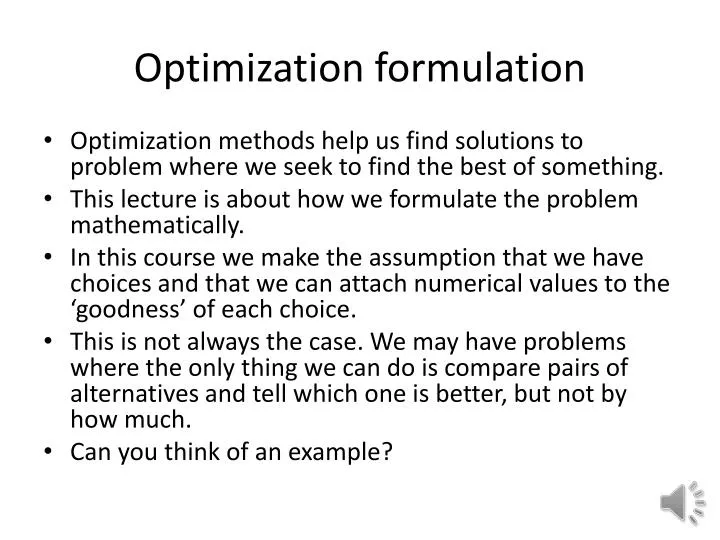
Optimization formulation • Optimization methods help us find solutions to problem where we seek to find the best of something. • This lecture is about how we formulate the problem mathematically. • In this course we make the assumption that we have choices and that we can attach numerical values to the ‘goodness’ of each choice. • This is not always the case. We may have problems where the only thing we can do is compare pairs of alternatives and tell which one is better, but not by how much. • Can you think of an example?
Young Modulus Example • The pairs (1,1), (2,2), (4,3) represent strain (millistrains) and stress (ksi) measurements. • Our model is , where is strain and is stress • We see to find E that will minimize the maximum difference between the data and the model. • E is our “design variable” and the maximum difference is the “objective function”
Direct unconstrained formulation • Minimize maximum difference eps=[1 2 4];sig=[1 2 3] e=linspace(0.5,1,101); sigmodel=e'*eps; sigr=ones(101,1)*sig; diff=abs(sigr-sigmodel); maxdiff=max(diff'); plot(e,maxdiff); xlabel('E'); ylabel('maximum difference'); • Non-smooth function • Difficult to optimize numerically.
Constrained formulation • To avoid a non-smooth function, a standard trick is to add a design variable b that bounds the difference, as well as two constraints • Note that the objective function is equal to one design variable, and the other variable E appears only in the constraints. • Not only is the new objective and constraints smooth, but they are also linear.
Standard notation • The standard form of an optimization problem used by most textbooks and software is • Standard form of Young’s modulus fit
Multiple objectives • It is common to have multiple objectives. • For fitting Young’s modulus, we may have also wanted to minimize the average absolute difference. avgdiff=mean(diff'); plot(e,maxdiff,avgdiff,'r') xlabel('E') legend('maxdiff','avgdiff','Location','north') Interval of interest is (0.75,0.83)
Column design example • Vanderplaats, Numerical optimization techniques for engineering design, 3rd edition.
In praise of normalization • The column design formulation has normalized constraints • Improves understanding: When equal to 0.1 we know it is 10% violation. • Improve numerical conditioning, because all constraints are of the same order of magnitude. • For same reason, it is good to normalize design variables when they are not all of the same order, like diameter and thickness.