Download
1 / 21
210 likes | 370 Vues
R. J. Rutten ‘Radiation transfer in stellar atmospheres ’ 2.6 NLTE. 2011.05.20 Tetsu Anan. non-LTE. 2. Non-local thermodynamical equilibrium ここでは、 Statistical equilibrium ○ Maxwell distribution ○ Complete redistribution (Χ ν =ψ ν =φ ν ) ○ Population ≠ local Saha-Boltzmann equilibrium.

E N D
R. J. Rutten‘Radiation transfer in stellar atmospheres ’2.6 NLTE 2011.05.20 Tetsu Anan
non-LTE 2 • Non-local thermodynamical equilibrium • ここでは、 • Statistical equilibrium ○ • Maxwell distribution ○ • Complete redistribution (Χν=ψν=φν) ○ • Population ≠ local Saha-Boltzmann equilibrium ψ: 自然放射の emission 確立分布 Χ : 誘導放射の profile shape φ : extinction profile
2.6.1 Statistical equilibrium 3 Rate equations i, j : エネルギー準位 減る量 増える量 Transition rates (Pij) = Radiative (Rij) + Collisional (Cij) (2.101) 詳細は3.2節で Transport equations 注目している遷移だけでなく、他準位間の遷移、 振動数によっては他の原子・分子の遷移(連続光なども)にも依存する
2.6.1 Statistical equilibrium 4 Time-dependent transfer. • dni/dt ≠ 0 のとき、粒子数を保存しながら時間変化する • 系統的なplasmaの流れ (=> ドップラーシフト => 方向によってαlineが違う) => 原泉関数が非等方になる • (Time-dependent??) 詳細は71ページで Multi-dimensional transfer. • 周辺媒質の不均一性 => 2 or 3次元の輻射輸送が必要 • テキストでは1次元 Mihalas & Mihalas 1984
2.6.2 NLTE descriptions 5 Departure coefficients nLTE : Saha-Boltzmann value NLTEの原因となるいろいろな影響を 丸め込んで表す 定義が定まってないから毎回定義に注意必要 Boltzmann distribution Saha-Boltzmann distribution Bound-bound のsource function、extinction Bound-free のsource function、extinction、emission、 free-free のsource function、extinction、emission をこれから紹介する
2.6.2 NLTE descriptions 6 Bound-bound source function ψ: 自然放射の emission 確立分布 Χ : 誘導放射の profile shape φ : extinction profile bl、bu Boltzman distribution Complete redistribution (Χν=ψν=φν )のとき、 Planck関数 Wien regime ( (bl/bu)exp(hν/kT) >>1 )のとき、
2.6.2 NLTE descriptions 7 Bound-bound extinction flu : classical dimensionless oscillator strength αlν= bl、bu Boltzman distribution (2.65) 散乱断面積表記 (2.66) Complete redistribution (Χν=ψν=φν )、Wien regimeのとき、 (2.98) (2.112) Total line extinction <<1 (Wien)
2.6.2 NLTE descriptions 8 Sνl<0 <= ανl <0 (自然放出) Laser = bu/bl T=10000K Laser regime Bu > bl 太陽ではMgⅠ (12um)など bu/bl 1 ν0
2.6.2 NLTE descriptions 9 Bound-free source function 添字 i : ionizing level c : level of the next stage of ionization (usually ground state) 自由電子の衝突捕獲は、Complete redistribution (Χν=ψν=φν ) i i Wien regime 運動エネルギー => 輻射エネルギー (2.118)
2.6.2 NLTE descriptions 10 Planck関数 Bound-free extinction bcはMaxwell分布で~1 Bound-free emission 水素様イオンのσνbf Wien part (hν>>kT) (2.74) (水素様イオンだと)〜exp(-hν/kT) Rayleigh-Jeans part (hν<<kT) The emissivity is not affected by lasering because the stimulated emission went to ανbf in (2.119) ?
2.6.2 NLTE descriptions 11 Edgeの話 Wien part (hν>>kT) では、emission edge is much sharper than the extinction edge. Fig. 2.6 exp(-hν/kT) ∝水素イオンのJ
2.6.2 NLTE descriptions 12 Free-free source function, extinction, emission Complete redistribution (Χν=ψν=φν ) Ionのpopulation 他の遷移からの影響 Free-free => 「Maxwell distribution for the kinetic energy => new bremsstrahlung photon」 Source function = Planck function
2.6.2 NLTE descriptions 13 Formal temperatures 「どのくらいnonLTEなのか」 指標として種々の温度Txは便利である TxとTeの違いをみる Excitation temperature Texc General line, complete redistribution
2.6.2 NLTE descriptions 14 Formal temperatures Ionization temperature Tion Bound-free Radiation temperature Trad Brightness temperature Tb Effective temperature Teff
2.6.3 Coherent scattering 15 • 散乱が重要な場所/波長で「nonLTE」になる • 一番扱い易い散乱光 • 等方散乱 • 単色(monochromatic)散乱 (Coherent scatteringと呼ぶ) • 厳密には非等方だがこれからは等方的として議論する • 例) • 自由電子のThomson散乱 • Bound-bound 遷移の共鳴(resonance)散乱 ドップラーシフトによる色の変化 は無視 電子 u u u l l l
2.6.3 Coherent scattering 16 Two-level atoms 波長は限定し空間的な非局所性だけ考える permits detailed discussion of spatial non-locality due to photon scattering process without spectral non-locality due to photon conversion processes. Bound-bound process Photon creation Photon scattering Photon destruction 右水平方向が 観測者 詳細は3.4.1で
2.6.3 Coherent scattering 17 Coherently scattering medium 単色、bound-boundの吸収係数は、 = photon destruction + photon scattering ちなみに、 連続光の吸収係数= 「(bound or free)-free」 + 「Thomson or Rayleigh scattering」 自由電子や粒子による光の散乱
2.6.3 Coherent scattering 18 Destruction probability 吸収(extinction)仮定において光子が破壊(destruction)される確立 吸収(extinction)仮定において光子が散乱される確立
2.6.3 Coherent scattering 19 r4 r5 Effective path, thickness, depth r3 r1 r6 光子が生成されて均質な媒質中をN回不規則に coherent scattering した実効的な距離 lν* (diffusion length, thermalization length, effective free path)は r2 lν* = (<(r1+r2+r3+r4+r5+・・・)2>)1/2〜N1/2 lν (2.137) ∵Nの平均=1/εν ∵(ανa) lν*=τν*、(ανa+ανs) lν =τν τν*〜1 光子が生成して散乱プロセスが始まった場所 τν〜1 光子が最後に散乱した場所 詳細は4.3節で
2.6.3 Coherent scattering 20 Source function 速度分布がMaxwellianのとき、 単色 two-level line source function = Planck 関数 pure coherent scattering (mean intensity に依存) Bound-free、free-free continuum processも同様 Complete redistribution (Χν=ψν=φν )のとき、
2.6.3 Coherent scattering 21 Transport equation 媒質がtwo-level atomsのとき、 太陽半径方向に軸対象、半径方向の光学的厚さτνを使うと、 (plane-parallel 大気)