Download
1 / 11
110 likes | 167 Vues
Explore how charges and currents determine electromagnetic waves, examining sources' impact on the wave properties. Learn the significance of small volume elements and the concept of retarded potentials. Understand the relationship between sources and the potentials' solutions in electromagnetic fields.

E N D
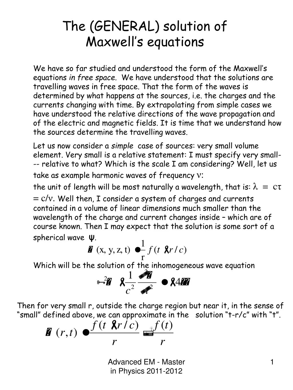
We have so far studied and understood the form of the Maxwell’s equations in free space. We have understood that the solutions are travelling waves in free space. That the form of the waves is determined by what happens at the sources, i.e. the charges and the currents changing with time.By extrapolating from simple cases we have understood the relative directions of the wave propagation and of the electric and magnetic fields. It is time that we understand how the sources determine the travelling waves. Let us now consider a simple case of sources: very small volume element. Very small is a relative statement: I must specify very small--- relative to what? Which is the scale I am considering? Well, let us take as example harmonic waves of frequency ν: the unit of length will be most naturally a wavelength, that is: λ = cτ = c/ν. Well then, I consider a system of charges and currents contained in a volume of linear dimensions much smaller than the wavelength of the charge and current changes inside – which are of course known. Then I may expect that the solution is some sort of a spherical wave ψ. Which will be the solution of the inhomogeneous wave equation The (GENERAL) solution of Maxwell’s equations Then for very small r, outside the charge region but near it, in the sense of “small” defined above, we can approximate in the solution “t-r/c” with “t”. Advanced EM - Master in Physics 2011-2012
Our job is to find the solution for the potentials once we know the sources: distributions of charge and of current. We could give the formula for the solution and just say that it is a solution, but we would rather like to understand that it is a solution and how can we find it. So now instead of starting from a s (source) and trying to findf(t-r/c) we will do the vice versa, i.e. try to find which s can generate a given f. Well, we already know that the function ψ(r,t)=f(t)/r satisfies the Poisson equation The situation is similar to the Poisson equation generated by a nearly pointlike source… a charge distribution over a tiny volume, such that So, if such a charge distribution satisfies the Poisson eq. with ρ then our equation for ψ(t)=f(t)/r (for r small). is a solution for r small of the equation Where s is a source of the time-variable potentials, it can be the charge distribution or one of the components of the current distribution. Carrying through the analogy, we have that Advanced EM - Master in Physics 2011-2012
The solution for small r is then We have found a solution valid for a small volume (in it the retardation term r/c is small compared to the typical “period” of the wave) of the time- varying equations. It turns out that it is a solution of the equation in which we have neglected the term We also know that f(t) is an approximation of f(t-r/c) for r/c small. It is at this point easy to generalize and write the general solution, also because we have learnt previously that the effect of the term: is to introduce the dependence on -r/c beside that on t In these equations, Φ (A)are the values of the potentials at the point r1at the instant t. They have been generated by the sources at point r2 at the earlier time t – r12/c, and are called Retarded Potentials Advanced EM - Master in Physics 2011-2012
They are called “Retarded Potentials” because the potential at the point where Iwant to know itand when I want to know it is retarded with respect to the time when it was generated. How is a retarded potential calculated? An essential condition for calculating a retarded potential is to know beforehand the motion of all charges – at least before the time at which we want to know the potential. Suppose we want to know the potential at the point O (that we choose as origin of the system of reference) and at the time t0. We have to find the time each charge generated the potential. We start sending light around backward in time at time t0 at the point O and take frames of the positions of charges at each spherical shell of thickness cδt: those which are within the shell of thickness cδt will contribute; we keep moving the radius of this anomalous light ray and keep adding up all the charge contributions that we find. I expect to find, in this process, a dependence on the velocity of the charges. Advanced EM - Master in Physics 2011-2012
Retarded potentials of a moving chargeor Lienard-Wiechert potentials Let β(r,t) J(r,t) be due to the motion in space of a charged particle. Where v is the velocity of the charge, which we assume to have a finite extension: a cube of side “a”. What we have to do now is to use the recipe given before for calculating the retarded potentials, i.e. have the spherical light shell moving backwards in time and intercepting ONCE the trajectory of the charge. Advanced EM - Master in Physics 2011-2012
The charge has to be spotted for times earlier and earlier as we move away from the Origin O that we have located where we wanted to compute the potentials. My light shell moving backwards in time in frames of thickness δtwill eventually get to intercept the moving charge at time t0. Since the charge has a finite size,it will take some finite time, however small, for the light to exit (at instant t1) from the other side of the charge volume. And… during this time the charge will have moved a bit. This “bit” is a distance, which we can call D, to indicate that it is a vector, So… the charge has radiated of course all the time. BUT, the radiated potential which has arrived to O at time t has been radiated between times t1 andt0, which is a different time than a/c! Advanced EM - Master in Physics 2011-2012
The distance over which what we have called the light pulse travelling back in time will have seen the moving charge (of side “a”) is L, with where the 2 equations are respectively the side of the charge cube plus the distance moved by the charge, and the distance moved by the light pulse during their transient crossing. is the unitary vector that from the position of the charge points towards the origin (i.e. where we are calculating the potentials). The calculation of the potentials includes an integration over the charge volume. But, as far as the integration of the 1/r term in the integral is concerned, the distance being anything – and usually much larger than the charge size- we can take 1/r out of the integral and consider it constant. We find with the last formula that the electrostatic potential q/R is modified by a factor L/a. To calculate it, we use the two formulas at the top of this page, to find that: And we have found the kinematical factor L/a which, as expected, depends on the velocity of the charge. Advanced EM - Master in Physics 2011-2012
We are now ready to calculate the retarded potential: If we want to calculate the potential in a point r1; and indicating with the sign ‘ “prime” the quantities computed at the time Don’t forget this one! It will come back over and over again. And it has a physical meaning! We obtain the equations: These are the Potentials of Lienard and Wiechert: to compute the fields, it is “sufficient” to compute their derivatives wrt time and the three space coordinates. Unfortunately, that “sufficient” which is a small problem from the general theoretical point of view, is not a simple problem at all in practice. Advanced EM - Master in Physics 2011-2012
Differentiating the Lienard-Wiechert potentials: the Lienard-Wiechert fields Writing the formulas for the fields once we have the expressions for the potentials is an easy business: Now, how do we calculate gradients and curls and time derivatives?? Simple, gradients and curls are also derivatives wrt space coordinates. Which space coordinates? We have r and r’ ...well, if we move r by δx there will be some “direct” derivatives, i.e. derivatives of r wrt x (y, z) but t’ and r’(t’) will also change. So, if I calculate the derivative wrt t of, say , v’ ,I will have to take into account the fact that moving “t” I will also move the point r’ and time t’ where the charge irradiates the potentials I am after. And I have to take into account that indirect variation as easily as possible, That will be done by writing: … and a similar treatment for gradient and curl. Advanced EM - Master in Physics 2011-2012
We know that From this formula we easily calculate is a bit more difficult to get, and we do it starting from the same formula for t’ in this page: But… wait a minute! This is just the kinematical factor dependent on the charge velocity that we obtained before with an euristic calculation! It is actually dt’/ dt ! It is coherent with the way we calculated it before: it is “how long does the charge radiate for an interval dt at the observer to differentiate the potential”. Now we must go on and differentiate t’ over space, i.e. compute the gradient of t’. That will be done in precisely the same way as we just did the ∂t’/ ∂t. We only have to derive the same formula for t’ wrt x (y,z) instead of t as we just did. Advanced EM - Master in Physics 2011-2012
In the formulas for the potentials, which we must derive, there are the following primed variables – which we have to derive wrt x,y,z and t:r’, v’,ε’. For them all we have to calculate the gradient and the derivative wrt to time t. Let us go on with ε’. We have now all the elements to calculate the most awkward element in the formulas of the potentials that we have to derivate: In this formula we notice the appearance (for the first time!) of the charge acceleration!!! We now have all the elements we need to write down in detail the fields: Eand B. Advanced EM - Master in Physics 2011-2012