Dynamic Mathematical Models in Process Engineering
Learn about essential mathematical models for theoretical processes with differential and algebraic equations explained. Understand the concept of state and output equations in vector form. Explore practical applications in heat exchange systems and linearization techniques.

Dynamic Mathematical Models in Process Engineering
E N D
Presentation Transcript
Chapter 2 Examples of Dynamic Mathematical Models Solution to Homework 2
Chapter 2 General Process Models State Equations • A suitable model for a large class of continuous theoretical processes is a set of ordinary differential equations of the form: t : Time variable x1,...,xn : State variables u1,...,um :Manipulated variables r1,...,rs :Disturbance, nonmanipulable variables f1,...,fn :Functions
Chapter 2 General Process Models Output Equations • A model of process measurement can be written as a set of algebraic equations: t : Time variable x1,...,xn : State variables u1,...,um :Manipulated variables rm1,...,rmt :Disturbance, nonmanipulable variables at output y1,...,yr : Measurable output variables g1,...,gr :Functions
Chapter 2 General Process Models State Equations in Vector Form • If the vectors of state variables x, manipulated variables u, disturbance variables r, and vectors of functions f are defined as: • Then the set of state equations can be written compactly as:
Chapter 2 General Process Models Output Equations in Vector Form • If the vectors of output variables y, disturbance variables rm, and vectors of functions g are defined as: • Then the set of algebraic output equations can be written compactly as:
Chapter 2 General Process Models Heat Exchanger in State Space Form Tl q V ρ T cp T q Tj If , then State Space Equations
Chapter 2 General Process Models Double-Pipe Heat Exchanger in State Space Form • Processes with distributed parameters are usually approximated by a series of well-mixed lumped parameter processes. • This is also the case for the heat exchanger, as shown in the next figure, which is divided into n well-mixed heat exchangers. • The space variable is divided into n equal lengths within the interval [0, L]. • After rearrangement, the mathematical model of the heat exchanger is of the form: • After rearrangement, the mathematical model of the heat exchanger is of the form: where and
Chapter 2 General Process Models Double-Pipe Heat Exchanger in State Space Form • We introduce the state parameters
Chapter 2 General Process Models Difference Quotient • The derivation with respect to space, δT/δτ, will now be approximated by using a difference quotient. • The difference quotient itself is the equation that can be used to approximately calculate the slope of a function at a certain point. • There are three formations of difference quotient: • Forward Difference • Backward Difference • Central Difference
Chapter 2 General Process Models Double-Pipe Heat Exchanger in State Space Form • Replacing δT/δτ with its corresponding difference will result a model that consists of a set of ordinary differential equations only: State Space Equations
Chapter 2 Linearization Linearization • Linearization is a procedure to replace a nonlinear original model with its linear approximation. • Linearization is done around a constant operating point. • It is assumed that the process variables change only very little and their deviations from steady state remain small. Operating point Linearization Taylor series expansion Nonlinear Model Linear Model
Chapter 2 Linearization Linearization • The approximation model will be in the form of state space equations • An operating point x0(t) is chosen, and the input u0(t) is required to maintain this operating point. • In steady state, there will be no state change at the operating point, or x0(t) = 0
Chapter 2 Linearization Taylor Expansion Series • Scalar Case A point near x0 Only the linear terms are used for the linearization
Chapter 2 Linearization Taylor Expansion Series • Vector Case where
Chapter 2 Linearization Taylor Expansion Series n: Number of states m : Number of inputs
Chapter 2 Linearization Taylor Expansion Series • Performing the same procedure for the output equations,
Chapter 2 Linearization Taylor Expansion Series r: Number of outputs
Chapter 2 Linearization Taylor Expansion Series Nonlinear Model Linear Model
Chapter 2 Linearization Single Tank System qi • The model of the system is already derived as: V h qo v1 • The relationship betweenh and h in the above equation is nonlinear. • An operating point for the linearization is chosen, (h0,qi,0).
Chapter 2 Linearization Single Tank System • The linearization around (h0,qi,0) for the state equation can be calculated as:
Chapter 2 Linearization Single Tank System • The linearization for the ouput equation is: • Note that the input of the linearized model is now Δqi. • To obtain the actual value of state and output, the following equation must be enacted:
Chapter 2 Linearization Single Tank System • The Matlab-Simulink model of the linearized system is shown below. All parameters take the previous values.
Chapter 2 Linearization Single Tank System • The simulation results : Original model : Linearized model
Chapter 2 Linearization Single Tank System • If the input qi deviates from the operating point, the linearized model will deliver inaccurate output. : Original model : Linearized model
Chapter 2 Linearization Single Tank System • If the input qi deviates from the operating point, the linearized model will deliver inaccurate output. : Original model : Linearized model
Chapter 2 Linearization Homework 3 Linearize the the interacting tank-in-series system for the operating point resulted by the parameter values as given in Homework 2. • For qi, use the last two digits of your Student ID. For example: 08 qi= 8 liters/s. • Submit the mdl-file and the screenshots of the Matlab-Simulink file + scope. qi h1 h2 q1 a1 a2 v2 v1
Chapter 2 Linearization Homework 3 (New) Linearize the the triangular-prism-shaped tank for the operating point resulted by the parameter values as given in Homework 2 (New). • For qi2, use the last two digits of your Student ID. For example: 03 qi2= 0.3 liter/s, 17 qi2= 1.7 liter/s. • Submit the mdl-file and the screenshots of the Matlab-Simulink file + scope. NEW qi2 qi1 hmax h a qo v