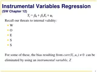
Instrumental Variables Regression (SW Chapter 12)
270 likes | 618 Vues
Instrumental Variables Regression (SW Chapter 12). Two Conditions for Valid Instrument. Estimation 1 of via 2SLS. IV Regression, Graphically. IV Regression, Algebraically. Example #1: Supply and demand. So we need a variable which shifts supply but not demand!.

Instrumental Variables Regression (SW Chapter 12)
E N D
Presentation Transcript
Ignoring endogeneity of ln(Price) . reg lpackpc lravgprs, r; Linear regression Number of obs = 48 F( 1, 46) = 38.86 Prob > F = 0.0000 R-squared = 0.4058 Root MSE = .18962 ------------------------------------------------------------------------------ | Robust lpackpc | Coef. Std. Err. t P>|t| [95% Conf. Interval] -------------+---------------------------------------------------------------- lravgprs | -1.213057 .1945897 -6.23 0.000 -1.604746 -.8213686 _cons | 10.33892 .9348204 11.06 0.000 8.457229 12.22062 ------------------------------------------------------------------------------
First stage 14
Combined 1st & 2nd stages YXZ . ivregress2sls lpackpc (lravgprs = rtaxso), vce(robust); Instrumental variables (2SLS) regression Number of obs = 48 Wald chi2(1) = 12.05 Prob > chi2 = 0.0005 R-squared = 0.4011 Root MSE = .18635 ------------------------------------------------------------------------------ | Robust lpackpc | Coef. Std. Err. z P>|z| [95% Conf. Interval] -------------+---------------------------------------------------------------- lravgprs | -1.083587 .3122035 -3.47 0.001 -1.695494 -.471679 _cons | 9.719876 1.496143 6.50 0.000 6.78749 12.65226 ------------------------------------------------------------------------------ Instrumented: lravgprs This is the endogenous X Instruments: rtaxso This is the instrumental variable • 2SLS is the estimator, as opposed to GMM or LIML • Don’t abbreviate as “ivreg”! Old “ivreg” command vs. “ivregress: http://www.ats.ucla.edu/stat/stata/seminars/stata10/endogenous.htm
Example: 1 instrument YWXZ . ivregress2slslpackpclperinc (lravgprs = rtaxso), vce(robust); Instrumental variables (2SLS) regression Number of obs = 48 Wald chi2(2) = 17.47 Prob > chi2 = 0.0002 R-squared = 0.4189 Root MSE = .18355 ------------------------------------------------------------------------------ | Robust lpackpc | Coef. Std. Err. z P>|z| [95% Conf. Interval] -------------+---------------------------------------------------------------- lravgprs | -1.143375 .3604804 -3.17 0.002 -1.849903 -.4368463 lperinc | .214515 .3018474 0.71 0.477 -.377095 .8061251 _cons | 9.430658 1.219401 7.73 0.000 7.040675 11.82064 ------------------------------------------------------------------------------ Instrumented: lravgprs Instruments: lperincrtaxso
Example: 2 instruments YWXZ1 Z2 . ivregress2slslpackpclperinc (lravgprs = rtaxsortaxs), vce(robust); Instrumental variables (2SLS) regression Number of obs = 48 Wald chi2(2) = 34.51 Prob > chi2 = 0.0000 R-squared = 0.4294 Root MSE = .18189 ------------------------------------------------------------------------------ | Robust lpackpc | Coef. Std. Err. z P>|z| [95% Conf. Interval] -------------+---------------------------------------------------------------- lravgprs | -1.277424 .2416838 -5.29 0.000 -1.751115 -.8037324 lperinc | .2804045 .2458274 1.14 0.254 -.2014083 .7622174 _cons | 9.894955 .9287578 10.65 0.000 8.074623 11.71529 ------------------------------------------------------------------------------ Instrumented: lravgprs Instruments: lperincrtaxsortaxs • Differences when multiple instruments? • Normal or inferior good? Luxury good or not? • Elastic or inelastic? 23