Download
1 / 27
270 likes | 285 Vues
This research aims to improve the precision of county-level data on tobacco use by using small area estimation techniques. It involves borrowing strength from relevant sources, combining information from multiple surveys, and utilizing model-based estimation approaches.

E N D
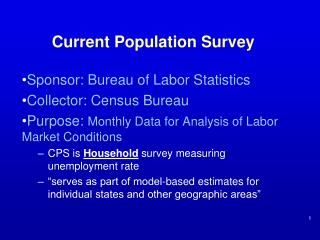
Small Area Estimation for the Tobacco Use Supplement to the Current Population Survey Benmei Liu Statistical Research and Applications Branch/ SRP/DCCPS May 10 2018 TCRB Scientific Staff Meeting
Outline • Overview of Small Area Estimation (SAE) • Research goals • SAE models and implementation • Model-based estimates – for maps • Summary and discussion
Why Small-Area Estimation? • The TUS-CPS is designed to produce reliable estimates at the national and state levels. • Policy makers, cancer control planners and researchers often need county level data for tobacco related measures in order to better evaluate tobacco control programs, monitor progress, and conduct tobacco-related research. • The standard direct estimation (design-based) methods for TUS data cannot provide reliable estimates at county level due to small (or zero) sample size • Model-based methods that combine information from multiple related sources are needed to increase precision
Overview of the Model-based SAE Techniques • Borrowing strength from relevant sources (Census/ Administrative information, related surveys) • Borrowed strength comes from covariates, and from other counties with similar characteristics • Methods of combining Information • Choose good small area model • Use good statistical methodology • Mixed models (fixed effects + random effects) at area level or unit level have been popularly used in the small area estimation literature (Rao 2003, Jiang and Lahiri 2006). • Among the many models developed in the SAE literature, the most prominent approach is the Fay-Herriot area- level model, originally developed to estimate per-capita income for U.S. areas with populations of less than 1,000.
Statistical Inferences Using Mixed Models • The final estimates are combinations of the direct estimates with the synthetic estimates. • Fully Bayesian approach or empirical best prediction approach (analytic formulas) can be used for the estimation.
Application of SAE Techniques in Estimating Proportions • Estimate cancer risk factors & screening behaviors for states and counties by combining data from Behavior Risk factor Surveillance System (BRFSS) and National Health Interview Survey (NHIS) (http://sae.cancer.gov/) • Estimate poverty rates for states, counties, and school districts in the Census Bureau’s Small Area Income and Poverty (SAIPE) program (http://www.census.gov/did/www/saipe/) • Estimate substance rates for states with data from the National Survey on Drug Use and Health (NSDUH) (http://www.samhsa.gov/data/NSDUH/2k11State/NSDUHsae2011/index.aspx) • Estimate proportions at the lowest level of literacy for states and counties with data from the National Assessment of Adult Literacy (NAAL) (http://nces.ed.gov/naal/estimates/overview.aspx)
Research Goals • Produce model-based, county level estimates (n=3,137) for the following key measures (2010/2011 TUS, age 18+): • Percent of population currently smoking • Percent of population that has ever smoked • Percent of population that has quit for 24+ hours, among those who have smoked within the past year • Percent of population governed by a smoke-free workplace policy • Percent of population governed by a smoke–free home rule • Involved collaboration among NCI, the Census Bureau, and the University of Maryland
Parameters of interest The population proportions: where is a binary response for unit k in county is the population total in county . Let denote the sample size, denote a vector of auxiliary variables.
Direct Estimates of and Associated Variances • Direct estimates (design-unbiased): • Variances of the direct estimates: =, . Where is the design effect reflecting the complex design (Kish 1965). • Problem of : Variance too large (imprecise estimates) for small sample sizes • Small area estimation techniques to address imprecise estimates
Commonly Used Area Level Model: Fay-Herriot Model The well known Fay-Herriot model (Fay & Herriot 1979): • Sampling model: • is the sampling variance and is assumed known • Linking model: where ; • This is equivalent to: where , ; • Several transformations on the direct estimates are proposed to stabilize sampling variance
Fay-Herriot Model with C&R Arcsin Transformation Let ; (Carter & Rolph, 1974 JASA) • Sampling model: • Linking model: where • Goal: To estimate • Model was chosen based on an extensive simulation study • Hyper parameters to be estimated are ,
Estimate the Design Effects • The design effect (or DEFF) is the ratio of the actual variance of a sample to the variance of a simple random sample of the same number of elements • Multiple ways can be used to estimate DEFF. • We used Kish’s traditional design effect formula given the clustering design of TUS-CPS, and estimated the state level design effects. We then used the state level DEFF to estimate the county level DEFF.
Auxiliary Variables • The pool of auxiliary variables include: • 30 county-level demographic & socio-economic variables obtained from ACS 2005-2009, 2008-2012, Census 2000 & 2010, and other administrative records; • 5 state level tobacco policy data (cigarette taxes, clean air laws, tobacco control funding, Medicaid Coverage for Tobacco-Related Treatment, year in which Quitline service was established) • Classical model selection procedures are applied to reduce the number of auxiliary variables for each outcome • Tested forcing in several strong unit level covariates: only worked for current smoking and smoking cessation.
Statistical Inference and Model Diagnosis • Hiearchical Bayesian approach through Markov Chain Monte Carlo (MCMC) methods were used to estimate the parameters of the statistical models. • Extensive model selection and model diagnosis procedures are used to select the final models and assess the goodness of fit for each model. • Modeled estimates were compared to the available direct estimates. The ratio of the two is expected to converge to 1 as the sample size gets larger.
Ratio of the Direct Over the Modeled Estimates for the Current Smoking Prevalence
Model-based vs Design-based Estimates for Current Smoking Prevalence –Maryland 2010/11
Model-based Estimates for Percent of Population Currently Smoking Among Age 18+: TUS-CPS 10/11
Model-based Estimates for Percent of Population Ever Smoked Among Age 18+: TUS-CPS 10/11
Model-based Estimates for Percent of Population Live in Smoke-Free Home Among Age 18+: TUS-CPS 10/11
Model-based Estimates for Percent of Population Attempt Quit Smoking for 24+ Hours Among Age 18+: TUS-CPS 10/11
Model-based Estimates for Percent of Population Governed by a Smoke-free Workplace Policy* Among Age 18+: TUS-CPS 10/11 Law Legislations Individual Self-Reported *Workplace has an official smoking policy: Smoking Not allowed in ANY public areas and work areas https://sae.cancer.gov/tus-cps/
Other Applications of SAE at NCI • Small Area Estimates for Cancer Risk Factors and Screening Behaviors by Combining multiple Surveys • Multiple years of state and county level estimates are produced for 7 variables • Utilize data from both the National Health Interview Survey and the Behavior Risk Factor Surveillance System • Small area estimates using the NCI-sponsored Health Information national Trends Survey (HINTS) • State level estimates are produced for 15 cancer-related knowledge variables • Spatio-temporal Models for Cancer Burden Mapping • To estimate age-standardized mortality rates and incidence rates by US county from a number of cancers and map the estimates to identify patterns and outliers
Summary and Discussion • More details and results are available at https://sae.cancer.gov/tus-cps/. • County level estimates of current and ever smoking prevalence derived from this project are available upon request. Similar estimates were derived from the combining NHIS/BRFSS project and released at https://sae.cancer.gov/nhis-brfss/. • Model-based SAE techniques represent a promising means of generating estimates where there is small (or zero) state or county sample. • The SAE results provide a useful resource for the cancer surveillance, evaluation, and research communities. • We are currently working on the TUS-CPS SAE estimates for the 2014/2015 data cycle. • Future works include model improvements and estimates for county by Race/ethnicity groups
Any Questions? Thank you! Contact info: Benmei Liu liub2@mail.nih.gov