Advanced Techniques in Software Pipelining and Code Optimization
This document explores software pipelining, a crucial concept in optimizing instruction execution within compilers. It covers the implementation of pipelining through iterations over arrays with specific arithmetic operations, showcasing efficient use of resources and minimizing execution latency. It delves into code scheduling, register allocation, and the application of precedence constraints to enhance performance. Additionally, it highlights static optimizations at compile-time to reduce hardware complexity, aiming to maintain high execution performance even on complex hardware setups.

Advanced Techniques in Software Pipelining and Code Optimization
E N D
Presentation Transcript
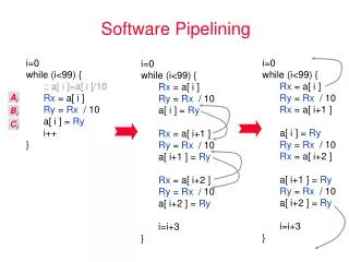
Software Pipelining i=0 while (i<99) { ;; a[ i ]=a[ i ]/10 Rx = a[ i ] Ry = Rx / 10 a[ i ] = Ry i++ } i=0 while (i<99) { Rx = a[ i ] Ry = Rx / 10 Rx = a[ i+1 ] a[ i ] = Ry Ry = Rx / 10 Rx = a[ i+2 ] a[ i+1 ] = Ry Ry = Rx / 10 a[ i+2 ] = Ry i=i+3 } i=0 while (i<99) { Rx = a[ i ] Ry = Rx / 10 a[ i ] = Ry Rx = a[ i+1 ] Ry = Rx / 10 a[ i+1 ] = Ry Rx = a[ i+2 ] Ry = Rx / 10 a[ i+2 ] = Ry i=i+3 } Ai Bi Ci
Software Pipelining (continued) i=0 while (i<99) { ;; a[ i ]=a[ i ]/10 Rx = a[ i ] Ry = Rx / 10 a[ i ] = Ry i++ } i=0 while (i<99) { Rx = a[ i ] Ry = Rx / 10 a[ i ] = Ry Rx = a[ i+1 ] Ry = Rx / 10 a[ i+1 ] = Ry Rx = a[ i+2 ] Ry = Rx / 10 a[ i+2 ] = Ry i=i+3 } i=0 Ry=a[ 0 ] / 10 Rx=a[ 1 ] while (i<97) { a[i]=Ry Ry=Rx / 10 Rx=a[i+2] i++ } a[97]=Ry a[98]=Rx / 10 Ai Bi Ci Ci Bi+1 Ai+2
Compiler Structure Frond End Optimizer Back End IR IR high-level source code machine code Dependence Analyzer Machine independent Machine dependent (IR= intermediate representation)
ASGI &d MULI INDIRI ADDI &a INDIRI INDIRI &b &c addi Rt1, Rb, Rc muli Rt2, Ra, Rt1 Code Selection Inst *match (IR *n) { • Map IR to machine instructions (e.g. pattern matching) switch (n->opcode) { case ……..: case MUL : l = match (n->left()); r = match (n->right()); if (n->type == D || n->type == F ) inst = mult_fp( (n->type == D), l, r ); else inst = mult_int ( (n->type == I), l, r); break; case ADD : l = match (n->left()); r = match (n->right()); if (n->type == D || n->type == F) inst = add_fp( (n->type == D), l, r); else inst = add_int ((n->type == I), l, r); break; case ……..: } return inst; }
Code Scheduling • Rearrange code sequence to minimize execution time • Hide instruction latency • Utilize all available resources
Register Allocation • Map virtual registers into physical registers • minimize register usage to reduce memory accesses • but introduces false dependencies . . . . .
• map virtual registers into architect registers • rearrange code • target machine specific optimizations - delayed branch - conditional move - instruction combining auto increment addressing mode add carrying (PowerPC) hardware branch (PowerPC) Instruction-level IR Back End IR Back End Machine code code code register code scheduling selection allocation emission
Code Scheduling • Objectives: minimize execution latency of the program • Start as early as possible instructions on the critical path • Help expose more instruction-level parallelism to the hardware • Help avoid resource conflicts that increase execution time • Constraints • Program Precedences • Machine Resources • Motivations • Dynamic/Static Interface (DSI): By employing more software (static) optimization techniques at compile time, hardware complexity can be significantly reduced • Performance Boost: Even with the same complex hardware, software scheduling can provide additional performance enhancement over that of unscheduled code
w[i+k].ip = z[i].rp + z[m+i].rp; w[i+j].rp = e[k+1].rp* (z[i].rp -z[m+i].rp) - e[k+1].ip * (z[i].ip - z[m+i].ip) ; FFT code fragment Precedence Constraints • Minimum required ordering and latency between definition and use • Precedence graph • Nodes: instructions • Edges (ab): a precedes b • Edges are annotated with minimum latency i1: l.s f2, 4(r2) i2: l.s f0, 4(r5) i3: fadd.s f0, f2, f0 i4: s.s f0, 4(r6) i5: l.s f14, 8(r7) i6: l.s f6, 0(r2) i7: l.s f5, 0(r3) i8: fsub.s f5, f6, f5 i9: f mul.s f4, f14, f5 i10: l.s f15, 12(r7) i11: l.s f7, 4(r2) i12: l.s f8, 4(r3) i13: fsub.s f8, f7, f8 i14: fmul.s f8, f15, f8 i15: fsub.s f8, f4, f8 i16: s.s f8, 0(r8)
Resource Constraints • Bookkeeping • Prevent resources from being oversubscribed
List Scheduling for Basic Blocks • Assign priority to each instruction • Initialize ready list that holds all ready instructions Ready = data ready and can be scheduled • Choose one ready instruction I from ready list with the highest priority Possibly using tie-breaking heuristics • Insert I into schedule Making sure resource constraints are satisfied • Add those instructions whose precedence constraints are now satisfied into the ready list
Priority Functions/Heuristics • Number of descendants in precedence graph • Maximum latency from root node of precedence graph • Length of operation latency • Ranking of paths based on importance • Combination of above
Orientation of Scheduling • Instruction Oriented • Initialization (priority and ready list) • Choose one ready instruction I and find a slot in schedule make sure resource constraint is satisfied • Insert I into schedule • Update ready list • Cycle Oriented • Initialization (priority and ready list) • Step through schedule cycle by cycle • For the current cycle C, choose one ready instruction I be sure latency and resource constraints are satisfied • Insert I into schedule (cycle C) • Update ready list
(a + b) * (c - d) + e/f 1 2 3 4 5 6 ld c ld a ld b ld d ld e ld f 7 8 9 fadd fsub fdiv 10 fmul load: 2 cycles add: 1 cycle sub: 1 cycle fadd 11 mul: 4 cycles div: 10 cycles orientation: cycle direction: backward heuristic: maximum latency to root List Scheduling Example
Scalar Scheduling Example green means candidate and ready red means candidate but not yet ready
Append the following to the previous example: *(p) =(x + Ry)- Rz ; p = p + 4 ; Take Home Example 12 16 ld x add fadd 13 14 fsub 15 s.f
Directions of List Scheduling • Backward Direction • Start with consumers of values • Heuristics • Maximum latency from root • Length of operation latency produces results just in time • Forward Direction • Start with producers of values • Heuristics • Maximum latency from root • Number of descendants • Length of operation latency produces results as early as possible
Limitations of List Scheduling • Cannot move instructions past conditional branch instructions in the program (scheduling limited by basic block boundaries) • Problem: Many programs have small numbers of instructions (4-5) in each basic block. Hence, not much code motion is possible • Solution: Allow code motion across basic block boundaries. • Speculative Code Motion: “jumping the gun” • execute instructions before we know whether or not we need to • utilize otherwise idle resources to perform work which we speculate will need to be done • Relies on program profiling to make intelligent decisions about speculation
Register Allocation • Mapping symbolic (virtual) registers used in IR onto architected (physical) registers • IR assumes unlimited number of symbolic registers • If the number of “live” values is greater than the number of physical registers in a machine, then some values must be kept in memory, i.e. we must insert spill code to “spill” some variables from registers out to memory and later reload them when needed Imagine if you only had one register • The objective in register allocation is to try to maximize keeping temporaries in registers and minimize memory accesses (spill code) maximize register reuse
Variable Live Range • A variable or value is “live”, along a particular control-flow path, from its definition to last use without any intervening redefinition • Live range, lr(x) • Group of paths in which x is live • Interference • x and y interfere if x and y are ever simultaneously alive along some control flow path i.e. lr(x) lr (y) y is not live x = y = =x =y =y
Nodes: live ranges Edges: interference beq r2 , $0 r1 r7 r6 r2 ld r5 , 24(r3) ld r4 , 16(r3) sub r6 , r2 , r4 add r2 , r1 , r5 sw r6 , 8(r3) r5 r3 r4 add r7 , r7 , 1 blt r7 , 100 Interference Graph r1, r2 & r3 are live-in “Live variable analysis” r1& r3 are live-out
Register Interference & Allocation • Interference Graph: G = <E,V> • Nodes (V) = variables, (more specifically, their live ranges) • Edges (E) = interference between variable live ranges • Graph Coloring (vertex coloring) • Given a graph, G=<E,V>, assign colors to nodes (V) so that no two adjacent (connected by an edge) nodes have the same color • A graph can be “n-colored” if no more than n colors are needed to color the graph. • The chromatic number of a graph is min{n} such that it can be n-colored • n-coloring is an NP-complete problem, therefore optimal solution can take a long time to compute How is graph coloring related to register allocation?
Chaitin’s Graph Coloring Theorem • Key observation: If a graph G has a node X with degree less than n (i.e. having less than n edges connected to it), then G is n-colorable IFF the reduced graph G’ obtained from G by deleting X and all its edges is n-colorable. Proof: G’ n-1 G
Graph Coloring Algorithm (Not Optimal) • Assume the register interference graph is n-colorable How do you choose n? • Simplification • Remove all nodes with degree less than n • Repeat until the graph has n nodes left • Assign each node a different color • Add removed nodes back one-by-one and pick a legal color as each one is added (2 nodes connected by an edge get different colors) Must be possible with less than n colors • Complications: simplification can block if there are no nodes with less than n edges Choose one node to spill based on spilling heuristic
C O L O R stack = {} C O L O R stack = {r5} r1 r7 r1 r7 remove r5 r2 r6 r2 r6 r5 r3 r3 r4 r4 remove r6 r1 r7 r1 r7 r2 remove r4 r2 r3 r3 r4 C O L O R stack = {r5, r6, r4} C O L O R stack = {r5, r6} Example (N = 5)
C O L O R stack = {} C O L O R stack = {r5} r1 r7 r7 r1 remove r5 r2 r6 r2 r6 r3 r3 r5 r4 r4 spill r1 Is this a ood choice?? r7 r7 r2 remove r6 r2 r6 r3 r3 r4 r4 C O L O R stack = {r5, r6} C O L O R stack = {r5} Example (N = 4) blocks
Register Spilling • When simplification is blocked, pick a node to delete from the graph in order to unblock • Deleting a node implies the variable it represents will not be kept in register (i.e. spilled into memory) • When constructing the interference graph, each node is assigned a value indicating the estimated cost to spill it. • The estimated cost can be a function of the total number of definitions and uses of that variable weighted by its estimated execution frequency. • When the coloring procedure is blocked, the node with the least spilling cost is picked for spilling. • When a node is spilled, spill code is added into the original code to store a spilled variable at its definition and to reload it at each of its use • After spill code is added, a new interference graph is rebuilt from the modified code, and n-coloring of this graph is again attempted
Phase Ordering Problem • Register allocation prior to code scheduling • false dependencies induced due to register reuse • anti and output dependencies impose unnecessary constraints • code motion unnecessarily limited • Code scheduling prior to register allocation • increase date live time (between creation and consumption) • overlap otherwise disjoint live ranges (increase register pressure) • may cause more live ranges to spill (run out of registers) • spill code produced will not have been scheduled One option: do both prepass and postpass scheduling.
[B. Rau & J. Fisher, 1993] Compiler/Hardware Interactions Front end & Optimizer Sequential (Superscalar) Determine Depend. Determine Depend. Dependence Architecture (Dataflow) Determine Independ. Determine Independ. Independence Architecture (Intel EPIC) Bind Resources Independence Bind Resources Architecture (Attached Array Processor) Execute DSI Hardware Compiler