Capital Budgeting Analysis
Capital Budgeting Analysis. Michael Bootsma Rachel Duschen Greg Ross. Cabernet-Merlot Project Overview. This presentation will walk you through my analysis of the proposed implementation of a new wine and give you my recommendation according to: NPV MIRR IRR Sensitivity Analysis.

Capital Budgeting Analysis
E N D
Presentation Transcript
Capital Budgeting Analysis Michael Bootsma Rachel Duschen Greg Ross
Cabernet-Merlot Project Overview • This presentation will walk you through my analysis of the proposed implementation of a new wine and give you my recommendation according to: • NPV • MIRR • IRR • Sensitivity Analysis
Key Base-Case Assumptions • The $333,000 outlay to rehabilitate the section of the main plant to be used in the making of the new wine is a sunk cost and therefore is not incorporated into the analysis
Key Base-Case Assumptions • The wholesale price and fixed cash operating costs were inflated at a constant rate of 2.8% and 5% accordingly for entire duration of the project. • The number of units expected to be sold in the first year is 171,500 units, determined by marketing and production managers
Key Base-Case Assumptions • A 3% T-bill rate and a 9.2% market risk premium were used in calculating the cost of capital • An asset beta of 1.79 and a capital structure of 44% debt and 56% equity were also used in formulating the cost of capital
Key Base-Case Assumptions • Depreciation is calculated according to 5-year MACRS • Machinery will have a $125,000 market value at the end of 8 years
Point of Controversy • An issue that evolved during the process of calculating final cash flow estimates was whether to include the effects of the new wine on the sales of existing wines • The amount of the decreased revenues was netted with the amount of decreased variable cash costs resulting in a $152,000 reduction in existing revenues
Key Figures • Expected Price per Unit = $38.50 • Receivables Factor = .125 • calculated using a 360-day year and Days Sales Outstanding ratio of 45 days • receivables will increase as a function of current-year sales • Variable Cost per Unit = $17.25
Key Figures • Variable Cost Payables Factor = .0428 • calculated using a 360-day year • 27% of variable costs represent credit purchases and are paid an average of 30 days later • the remaining 73% of variable costs consist of wages which are paid an average of 10 days later
Key Figures • Annual Cash Fixed Costs = $795,000 • Fixed Cost Payables Factor = .0542 • calculated using a 360-day year • 65% of fixed costs are paid for with credit and are paid an average of 30 days later • 35% of fixed costs are paid immediately
Key Figures • Opportunity Cost of Capital = 19% • calculated using the Asset Beta Model, which consists of adding the risk-free rate to the market risk premium multiplied by the asset beta • Sales in Years 2-5 are projected to be 35% higher than in Year 1 • Sales in Years 6-8 are projected to be 19% higher than in Year 1
Key Figures • Initial Investment = $4,100,000 • includes: • new machinery costing $3,700,000 • shipping and installation charges of $400,000 • Income Tax Rate = 30% • Initial Change in NWC= $288,000
Year 0 = - $4,218,293 Year 1 = $1,355,290 Year 2 = $3,003,712 Year 3 = $3,137,237 Year 4 = $3,012,215 Year 5 = $2,959,870 Year 6 = $2,582,466 Year 7 = $2,340,491 Year 8 = $3,223,669 Resulting Net Cash Flow Estimates-Base-Case
Final Estimates-Base Case • NPV = $5,897,016 • MIRR = 33.3% • IRR = 54.9%
Sensitivity Analysis • For every 5,000 change in unit sales there is an increase of $359,696 in NPV • For every $2 change in price there is an increase of $1,154,535 in NPV • For every $1 change in variable cost there is a decrease of $573,172 in NPV • Changes in price and cost inflation are insignificant along with a percent change in Cost of Capital
Scenario Analysis • In the worst case, 40,000 units would be sold and the price per bottle would be $20 • NPV = $(4,449,304) • Probability = 15%
Scenario Analysis • In the base-case, 171,500 were assumed to be sold • NPV = $5,885,865 • Probability = 70%
Scenario Analysis • In the best case, 244,500 units would be sold, causing variable cash operating costs to rise to $20 per unit • NPV = $8,890,280 • Probability = 15%
Scenario Analysis • By multiplying each NPV by its respective probability, the expected NPV is found to be $4,786,252 • The deviation was calculated to be $4,020,844
Risks • The worst case scenario would result in significant losses • The project is extremely sensitive to unit sales and price fluctuations • One deviation could nearly eliminate the positive NPV • Key Base-Case Assumptions could fluctuate
Recommendation • Our recommendation is to accept the Project • The Base Case NPV is positive • The IRR and MIRR are also Positive for the Base Case • The Cash flows are also substantial when compared to the initial investment
Recommendation Cont. • The Best Case Scenario presents a chance to almost double our NPV • The product is superior and would help expand our market share • The risks are justified with the potential returns • The company is well established and can assume the risks involved