Download
1 / 23
230 likes | 325 Vues
This study provides an overview of available data from several Swiss sites, focusing on the influence of topographic features on seismic response. It examines issues related to "polluted" noise and conducts topographic amplification studies based on earthquake response spectra. The research combines numerical simulations with recorded data to analyze the effects of altitude, slope, and natural frequencies on amplification. With a focus on Eurocode 8 categories, the study measures kappa from response spectra to understand attenuation effects. Various modelling examples, including unstable rockslope scenarios, are presented to demonstrate the impact of topography on seismic behavior.

E N D
FLACH X
FLACH 4 Hz
WILA X
WILA 5 Hz
WILA Relatively strong attenuation
BALST X
BALST 2.5 Hz
AIGLE X
DAVOX X
DAVOX 1.5 Hz
Issues INTR - N “polluted” noise
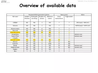
Topographic amplification studies based on earthquake resposne spectra (C. Cauzzi, SED) Combined used of numerical simulations (Sulmona, Irpinia) and recorded data; Relating topographic amplification with the local altitude, slope, and estimated natural frequencies of the relief; Focus on main topographic categories of the Eurocode 8 for station selection (data from CH, IT and JP); Measure kappa from response spectra to understand the role of attenuation on the observed amplification;
Next steps • WCEE abstract submitted (though the deadline for the paper submission is approaching …) • Common processing tools for polarization analysis: • What should we compare? (frequencies, angles + uncertainties) • What should we do with earthquake data? • kappa (Carlo) • polarization – comparison with noise results • ??? • Shallow geophysics - Active Noise correlation with D arrays (Cecile?) • Work on DEM models (comparison with INGV Milan – V. Pessina)
Modelling of unstable rockslopes (extreme case - Randa) 3Hz (Burjanek et al., GJI, 2010 Moore et al., BSSA, 2011)
Modelling of unstable rockslopes (extreme case - Randa) • FE element modelling of eigen-modes • Effective elastic properties (Vs=900m/s) necessary to fit eigen-frequency of 3Hz (Burjanek et al., ESG, 2011)
Modelling of unstable rockslopes (extreme case) • simulations of model wit cracks perfromed with UDEC (Moore et al., BSSA, 2011)
Modelling of unstable rockslopes (extreme case - Randa) Modelled site-to-reference s. ratio Modelled crack displacement Observed crack displacement Observed site-to-reference s. ratio (Moore et al., BSSA, 2011)
Modelling of unstable rockslopes (extreme case - Rawilhorn) • 1946 M6 Earthquake doublet (separated by 4 months) • Second event triggered the rockfall
Modelling of unstable rockslopes (extreme case - Rawilhorn) After M6.1 earthquake (Moore et al., ISL, 2012)