Sparse Table Implementation of Priority Queue for Efficient Data Management
This document presents a sparse table implementation of a priority queue (PQ), designed by Yaniv Nahum and written by Alon Itai, Alan G. Konheim, and Michael Rodeh. The sparse table approach allows efficient operations, including Search, Insert, Delete, Min, and Next, utilizing a linear array structure supported by dummy keys to enhance performance. By employing gaps in the table and sophisticated reconfiguration strategies, we achieve average-case performance improvements, making it suitable for practical applications where traditional tree-based structures fall short.


Sparse Table Implementation of Priority Queue for Efficient Data Management
E N D
Presentation Transcript
A sparse Table implementation of Priority Queue Presented by: Yaniv Nahum Written by: Alon Itai Alan G. Konheim Michael Rodeh
PQ - introduction • A data structure with the following operations: • Search (x) • Insert (x) • Delete (x) • Min • Next (x) • Scan
PQ - introduction • Most implementations use trees (2-3, AVL, weight balanced trees) and requires no more than O (log n) time. • In many cases, the algorithms devote much of their running time and storage manipulating the PQ, often rendering a theoretically efficient algorithm to infeasible or inefficient to all practical purposes.
PQ as Sparse table • Data is stored in linear array, and requires only one pointer. • Insertion requires: • Searching. • Moving (shifting of records). • Reconfiguring (increase size and distribute keys).
Performance • Assuming a table of size m. • Searching takes O (log m). • Move takes O (m) in worst case. • We will show that the expected number of moves is constant. • We will present a more complicated table, in order to improve worst case, which takes O (n*log^2(n)) to build.
Sparse table schemata • Records are stored in a sorted order. • Insertion is improved by introducing gaps in the table, thereby storing n records in a table of capacity m for some m > n. • m-n keys are dummy keys.
example • Genuine keys are located at addresses 2,5,6,8 in the following table: • y = (2,2,2,3,3,3,4,5,5). • n = 4. • m = 9.
Building a table • Determined by 2 sequences of real numbers: • {nk: 0<=k<INFINITY} • {mk: 1<=k<INFINITY} • 1=n0 < n1 < … < … • nk <= nk-1*mk 1<=k
Building a table • The size of the table, m, can only take the values nk-1*mk for k=1,2,… • The size of the table is m=nk-1*mk when the number of distinct keys in the table, n, satisfies nk-1<n<=nk
Insertion • Inserting x into a table of size m=nk-1*mk containing nk-1<n<=nk genuine keys find address s satisfying ys-1<x<=ys • If ys is a dummy key, it is replaced by x, yielding the table: (y0,…,ys-1,x,ys+1,…ym-1) • If ys is a genuine key, the block of t consecutive genuine keys is shift right one position.
Insertion (Cont …) • X is inserted at address s yielding the table: • (y0,…,ys-1,x,ys,…,ys+t-1,ys+t+1,…,ym-1) • Note: ys+t is the dummy key removed from table.
reconfiguration • When inserting x to a table with size m=nk-1*mk, and there are nk genuine keys. • The size of the table first increases to nk*mk+1, and the nk genuine keys are uniformly distribute in it. • Than, x is inserted regularly.
Some Insight … • The numbers {mk} are the expansion factors. • The ratio r = n / nk-1*mk with nk-1<n<=nk is the density of the genuine keys in the table. • 1 / mk < r <= 1 • mk adds log(mk) steps to the binary search but reduces the number of keys which must be moved to insert a new key.
Some Insight … • The cost of reconfiguration is O(nk*mk+1) if the number of keys inserted since the last reconfiguration, nk-nk-1, is proportional to the size of the expanded table, the cost of reconfiguration per key is constant.
Some Insight … • Worst case for insertion is O(n). We will show next that the expected number of moves remains bounded as nk increases (provided r is bounded away from 1).
Average behavior of S.T. • Proof …
Some theorems … • Theorem 1: On insertion (no deletion) the average number of move operations is bounded by a constant. • Theorem 2: On the average, insertion requires O(log n) operations. • Proof: search takes O(log m)=O(log n). The expected number of moves is constant. Reconfiguration adds only constant time per insertion.
Improving worst case • Worst case for insertion may be quite bad. • To improve w.c. performance, an additional structure is imposed to the sparse table. • The basic idea is to redistribute the keys locally when the local density become high.
Improving worst case • h = log m – log log m • b = m / 2^h • log m <= b < 2 log m • We divide the table into m/b = 2^h blocks B0,B1,…,B2^h-1 • We shall build a full binary tree of height h with leaves L0,L1,…,L2^h-1.
Improving worst case • Each node v wil have a segment s(v) as follows: • Leaf Li associate the block Bi (0<=i<2^h) • Node with children u and w: s(v) = s(u) U s(w) • m(v) is the size of s(v) • r(v) is the density, the number of geniune keys in s(v) divided by m(v).
Improving worst case • The nodes of the tree are divided into levels. The root r is at level 0, and the level of any other node is greater by one than that of it’s parent. • The level of the leaves is obviously h.
Improving worst case • Let 0<=tL<tU<=1. • We define the sequence t0,t1,…,th of threshold densities of nodes in levels 0,1,…,h by: tq=tL+q(tU-tL)/h 0<=q<=h • tL = t0 < t1 < … < th = tU • tq+1 – tq = (tU-tL)/h • r(Li) <= th during the process of insertion.
Insertion Algorithm • Insert the new key as in the previous algorithm. • If the density of Bi <= th, then insertion completed. • Otherwise, find the maximal level q for which r(vq)<tq. • If such q is found, then the genuine keys are uniformly distributed. • If q is not found, the table size is increased.
Theorem 3 • Performing n-nk-1 insertions into a sparse table of size m=nk-1mk requires at most O((n-nk-1)log^2(m/(tU-tL)) ) • Proof …
deletions • Deletions are easy to implement, but are difficult to analyze statitically. • In addition to the regular reconfiguration, reconfiguration will also occur whenever deletion reduces the number of genuine keys to some threshold. • The authors were not able to provide an analysis od s.t. under a sequence of insertions/deletions.