6.4 Partial Differential Equation
6.4 Partial Differential Equation. 指導老師:戴天時教授 學 生:王薇婷. The Feynman-Kac Theorem Previous section:. Convergences slowly. Numerical algorithm. the Euler method. Gives the function value for only one pair ( t, x). Convergences quickly. Gives the function for all value of ( t, x).

6.4 Partial Differential Equation
E N D
Presentation Transcript
6.4 Partial Differential Equation 指導老師:戴天時教授 學 生:王薇婷
The Feynman-Kac Theorem • Previous section: Convergences slowly Numerical algorithm the Euler method Gives the function value for only one pair ( t, x) Convergences quickly Gives the function for all value of ( t, x)
The general principle behind the proof of the Feynman-Kac theorem is: • Find the martingale • Take the differential • Set the dt term equal to zero
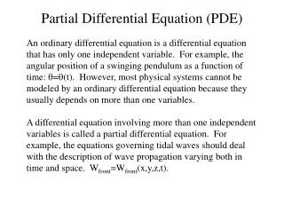
When the underlying asset is a geometric Brownian motion, this is the right pricing equation for a European Call, a European Put, a forward contract, and any other option that pays off some function of S(T) at time T. • The SDE for the underlying asset is (6.4.7) rather than (6.4.6). Because the conditional expectation in (6.4.8) under the risk-neutral measure and hence must use the differential equation .
The stock price would no longer be a geometric Brownian motion and the Black-Scholes-Merton formula would no longer apply. • It has been observed in markets that if one assumes a constant volatility, the parameter σ that makes the theoretical option price given by (6.4.9) agree with the market price, the so called implied volatility , is different options having different strikes. convex function volatility smile
One simple model with non-constant volatility is the constant elasticity of variance (CEV) model, in which depends on x but not t. the parameter is chosen so that the model gives a good fit to option prices across different strikes at a single expiration date. • The volatility is a decreasing function of the stock price.
When one wishes to account for different volatilities implied by options expiring at different dates as well as different strikes, one needs to allow σ to depend on t as well as x . This function σ(t ,x) is called the volatility surface.