PARTIAL DIFFERENTIAL EQUATIONS
PARTIAL DIFFERENTIAL EQUATIONS. Introduction. Given a function u that depends on both x and y , the partial derivatives of u w.r.t. x and y are:.


PARTIAL DIFFERENTIAL EQUATIONS
E N D
Presentation Transcript
Introduction • Given a function u that depends on both x and y, the partial derivatives of u w.r.t. x and y are:
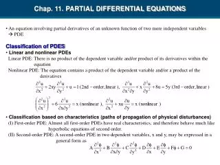
An equation involving partial derivatives of an unknown function of two or more independent variables is called Partial Differential Equation (PDE). Examples: The order of a PDE is that of the highest-order partial derivative appearing in the equation.
A PDE is linear if it is linear in the unknown function and all its derivatives, with coefficients depending only on the independent variables • e.g. x’’ + ax’ + bx + c = 0 – linear x’ = t2x – linear x’’ = 1/x – nonlinear
For linear, two independent variables second order equations can be expressed as: • where A, B and C are functions of x and y and D is a function of x, y, ¶u/¶x and ¶u/¶y. • Above equation can be classified into categories in the next slide based on values of A, B, and C.
Elliptic Equations • Typically used to characterize steady-state distribution of an unknown in two spatial dimensions.
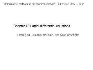
Laplace Equation The PDE as an expression of the conservation of energy
Need to reformulate the equation in terms of temperature. Use Fourier’s Law: and substituting back results in (Laplace equation)
Parabolic Equations • Heat conduction Hot Cool Heat balance (the amount of heat stored in the element) over a unit time, Dt
Input – Output = Storage Dividing by volume of the element (DxDyDz) and Dt Taking the limit yields:
Substituting Fourier’s Law: Gives:
Solution • Finite Difference A grid used for the finite difference solution of elliptic PDEs in two independent variables.
Numerical Differentiation using Centred-Finite Divided Difference • First Derivative • Second Derivative • Third Derivative
Solution • Finite Element
Finite Element Analysis • Two interpretations • Physical Interpretation: The continous physical model is divided into finite pieces called elements and laws of nature are applied on the generic element. The results are then recombined to represent the continuum. • Mathematical Interpretation: The differentional equation representing the system is converted into a variational form, which is approximated by the linear combination of a finite set of trial functions.