Lecture 10 Clustering
Lecture 10 Clustering. Preview. Introduction Partitioning methods Hierarchical methods Model-based methods Density-based methods. Examples of Clustering Applications.

Lecture 10 Clustering
E N D
Presentation Transcript
Preview • Introduction • Partitioning methods • Hierarchical methods • Model-based methods • Density-based methods
Examples of Clustering Applications • Marketing: Help marketers discover distinct groups in their customer bases, and then use this knowledge to develop targeted marketing programs • Land use: Identification of areas of similar land use in an earth observation database • Insurance: Identifying groups of motor insurance policy holders with a high average claim cost • Urban planning: Identifying groups of houses according to their house type, value, and geographical location • Seismology: Observed earth quake epicenters should be clustered along continent faults
What Is a Good Clustering? • A good clustering method will produce clusters with • High intra-class similarity • Low inter-class similarity • Precise definition of clustering quality is difficult • Application-dependent • Ultimately subjective
Requirements for Clustering in Data Mining • Scalability • Ability to deal with different types of attributes • Discovery of clusters with arbitrary shape • Minimal domain knowledge required to determine input parameters • Ability to deal with noise and outliers • Insensitivity to order of input records • Robustness wrt high dimensionality • Incorporation of user-specified constraints • Interpretability and usability
Similarity and Dissimilarity Between Objects • Same we used for IBL (e.g, Lp norm) • Euclidean distance (p = 2): • Properties of a metric d(i,j): • d(i,j) 0 • d(i,i)= 0 • d(i,j)= d(j,i) • d(i,j) d(i,k)+ d(k,j)
Major Clustering Approaches • Partitioning: Construct various partitions and then evaluate them by some criterion • Hierarchical: Create a hierarchical decomposition of the set of objects using some criterion • Model-based: Hypothesize a model for each cluster and find best fit of models to data • Density-based: Guided by connectivity and density functions
Partitioning Algorithms • Partitioning method: Construct a partition of a database D of n objects into a set of k clusters • Given a k, find a partition of k clusters that optimizes the chosen partitioning criterion • Global optimal: exhaustively enumerate all partitions • Heuristic methods: k-means and k-medoids algorithms • k-means (MacQueen, 1967): Each cluster is represented by the center of the cluster • k-medoids or PAM (Partition around medoids) (Kaufman & Rousseeuw, 1987): Each cluster is represented by one of the objects in the cluster
K-Means Clustering • Given k, the k-means algorithm consists of four steps: • Select initial centroids at random. • Assign each object to the cluster with the nearest centroid. • Compute each centroid as the mean of the objects assigned to it. • Repeat previous 2 steps until no change.
K-Means Clustering (contd.) • Example
Comments on the K-Means Method • Strengths • Relatively efficient: O(tkn), where n is # objects, k is # clusters, and t is # iterations. Normally, k, t << n. • Often terminates at a local optimum. The global optimum may be found using techniques such as simulated annealing and genetic algorithms • Weaknesses • Applicable only when mean is defined (what about categorical data?) • Need to specify k, the number of clusters, in advance • Trouble with noisy data and outliers • Not suitable to discover clusters with non-convex shapes
Step 0 Step 1 Step 2 Step 3 Step 4 agglomerative (AGNES) a a b b a b c d e c c d e d d e e divisive (DIANA) Step 3 Step 2 Step 1 Step 0 Step 4 Hierarchical Clustering • Use distance matrix as clustering criteria. This method does not require the number of clusters k as an input, but needs a termination condition
AGNES (Agglomerative Nesting) • Produces tree of clusters (nodes) • Initially: each object is a cluster (leaf) • Recursively merges nodes that have the least dissimilarity • Criteria: min distance, max distance, avg distance, center distance • Eventually all nodes belong to the same cluster (root)
A Dendrogram Shows How the Clusters are Merged Hierarchically • Decompose data objects into several levels of nested partitioning (tree of clusters), called a dendrogram. • A clustering of the data objects is obtained by cutting the dendrogram at the desired level. Then each connected component forms a cluster.
DIANA (Divisive Analysis) • Inverse order of AGNES • Start with root cluster containing all objects • Recursively divide into subclusters • Eventually each cluster contains a single object
Other Hierarchical Clustering Methods • Major weakness of agglomerative clustering methods • Do not scale well: time complexity of at least O(n2), where n is the number of total objects • Can never undo what was done previously • Integration of hierarchical with distance-based clustering • BIRCH: uses CF-tree and incrementally adjusts the quality of sub-clusters • CURE: selects well-scattered points from the cluster and then shrinks them towards the center of the cluster by a specified fraction
BIRCH • BIRCH: Balanced Iterative Reducing and Clustering using Hierarchies (Zhang, Ramakrishnan & Livny, 1996) • Incrementally construct a CF (Clustering Feature) tree • Parameters: max diameter, max children • Phase 1: scan DB to build an initial in-memory CF tree (each node: #points, sum, sum of squares) • Phase 2: use an arbitrary clustering algorithm to cluster the leaf nodes of the CF-tree • Scales linearly: finds a good clustering with a single scan and improves the quality with a few additional scans • Weaknesses: handles only numeric data, sensitive to order of data records.
Clustering Feature:CF = (N, LS, SS) N: Number of data points LS: Ni=1 Xi SS: Ni=1 Xi2 Clustering Feature Vector CF = (5, (16,30),(54,190)) (3,4) (2,6) (4,5) (4,7) (3,8)
CF1 CF2 CF3 CF6 child1 child2 child3 child6 CF Tree Root B = 7 L = 6 Non-leaf node CF1 CF2 CF3 CF5 child1 child2 child3 child5 Leaf node Leaf node prev CF1 CF2 CF6 next prev CF1 CF2 CF4 next
CURE (Clustering Using REpresentatives) • CURE: non-spherical clusters, robust wrt outliers • Uses multiple representative points to evaluate the distance between clusters • Stops the creation of a cluster hierarchy if a level consists of k clusters
Drawbacks of Distance-Based Method • Drawbacks of square-error-based clustering method • Consider only one point as representative of a cluster • Good only for convex clusters, of similar size and density, and if k can be reasonably estimated
Cure: The Algorithm • Draw random sample s • Partition sample to p partitions with size s/p • Partially cluster partitions into s/pq clusters • Cluster partial clusters, shrinking representatives towards centroid • Label data on disk
y y y x y y x x Data Partitioning and Clustering • s/pq = 5 • s = 50 • p = 2 • s/p = 25 x x
y y x x Cure: Shrinking Representative Points • Shrink the multiple representative points towards the gravity center by a fraction of . • Multiple representatives capture the shape of the cluster
Model-Based Clustering • Basic idea: Clustering as probability estimation • One model for each cluster • Generative model: • Probability of selecting a cluster • Probability of generating an object in cluster • Find max. likelihood or MAP model • Missing information: Cluster membership • Use EM algorithm • Quality of clustering: Likelihood of test objects
Mixtures of Gaussians • Cluster model: Normal distribution (mean, covariance) • Assume: diagonal covariance, known variance, same for all clusters • Max. likelihood: mean = avg. of samples • But what points are samples of a given cluster? • Estimate prob. that point belongs to cluster • Mean = weighted avg. of points, weight = prob. • But to estimate probs. we need model • “Chicken and egg” problem: use EM algorithm
EM Algorithm for Mixtures • Initialization: Choose means at random • E step: • For all points and means, compute Prob(point|mean) • Prob(mean|point) = Prob(mean) Prob(point|mean) / Prob(point) • M step: • Each mean = Weighted avg. of points • Weight = Prob(mean|point) • Repeat until convergence
EM Algorithm (contd.) • Guaranteed to converge to local optimum • K-means is special case
AutoClass • Developed at NASA (Cheeseman & Stutz, 1988) • Mixture of Naïve Bayes models • Variety of possible models for Prob(attribute|class) • Missing information: Class of each example • Apply EM algorithm as before • Special case of learning Bayes net with missing values • Widely used in practice
COBWEB • Grows tree of clusters (Fisher, 1987) • Each node contains: P(cluster), P(attribute|cluster) for each attribute • Objects presented sequentially • Options: Add to node, new node; merge, split • Quality measure: Category utility: Increase in predictability of attributes/#Clusters
Neural Network Approaches • Neuron = Cluster = Centroid in instance space • Layer = Level of hierarchy • Several competing sets of clusters in each layer • Objects sequentially presented to network • Within each set, neurons compete to win object • Winning neuron is moved towards object • Can be viewed as mapping from low-level features to high-level ones
Self-Organizing Feature Maps • Clustering is also performed by having several units competing for the current object • The unit whose weight vector is closest to the current object wins • The winner and its neighbors learn by having their weights adjusted • SOMs are believed to resemble processing that can occur in the brain • Useful for visualizing high-dimensional data in 2- or 3-D space
Density-Based Clustering • Clustering based on density (local cluster criterion), such as density-connected points • Major features: • Discover clusters of arbitrary shape • Handle noise • One scan • Need density parameters as termination condition • Representative algorithms: • DBSCAN (Ester et al., 1996) • DENCLUE (Hinneburg & Keim, 1998)
p MinPts = 5 Eps = 1 cm q Definitions (I) • Two parameters: • Eps: Maximum radius of neighborhood • MinPts: Minimum number of points in an Eps-neighborhood of a point • NEps(p) ={q Є D | dist(p,q) <= Eps} • Directly density-reachable: A point p is directly density-reachable from a point q wrt. Eps, MinPts iff • 1) p belongs to NEps(q) • 2) q is a core point: |NEps (q)| >= MinPts
p q o Definitions (II) • Density-reachable: • A point p is density-reachable from a point q wrt. Eps, MinPts if there is a chain of points p1, …, pn, p1 = q, pn = p such that pi+1 is directly density-reachable from pi • Density-connected • A point p is density-connected to a point q wrt. Eps, MinPts if there is a point o such that both, p and q are density-reachable from o wrt. Eps and MinPts. p p1 q
Outlier Border Eps = 1cm MinPts = 5 Core DBSCAN: Density Based Spatial Clustering of Applications with Noise • Relies on a density-based notion of cluster: A cluster is defined as a maximal set of density-connected points • Discovers clusters of arbitrary shape in spatial databases with noise
DBSCAN: The Algorithm • Arbitrarily select a point p • Retrieve all points density-reachable from p wrt Eps and MinPts. • If p is a core point, a cluster is formed. • If p is a border point, no points are density-reachable from p and DBSCAN visits the next point of the database. • Continue the process until all of the points have been processed.
DENCLUE: Using Density Functions • DENsity-based CLUstEring (Hinneburg & Keim, 1998) • Major features • Good for data sets with large amounts of noise • Allows a compact mathematical description of arbitrarily shaped clusters in high-dimensional data sets • Significantly faster than other algorithms (faster than DBSCAN by a factor of up to 45) • But needs a large number of parameters
DENCLUE • Uses grid cells but only keeps information about grid cells that do actually contain data points and manages these cells in a tree-based access structure. • Influence function: describes the impact of a data point within its neighborhood. • Overall density of the data space can be calculated as the sum of the influence function of all data points. • Clusters can be determined mathematically by identifying density attractors. • Density attractors are local maxima of the overall density function.
Influence Functions • Example
Clustering: Summary • Introduction • Partitioning methods • Hierarchical methods • Model-based methods • Density-based methods