Fall 2004, CIS, Temple University CIS527: Data Warehousing, Filtering, and Mining Lecture 3 Data Warehousing and OLAP Te

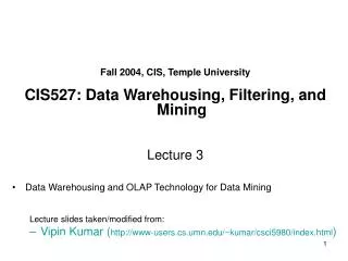
1. Fall 2004, CIS, Temple University CIS527: Data Warehousing, Filtering, and Mining Lecture 3 • Data Warehousing and OLAP Technology for Data Mining Lecture slides taken/modified from: • Vipin Kumar (http://www-users.cs.umn.edu/~kumar/csci5980/index.html)

2. What is Data? • Collection of data objects and their attributes • An attribute is a property or characteristic of an object • Examples: eye color of a person, temperature, etc. • Attribute is also known as variable, field, characteristic, or feature • A collection of attributes describe an object • Object is also known as record, point, case, sample, entity, or instance Attributes Objects

3. Attribute Values • Attribute values are numbers or symbols assigned to an attribute • Distinction between attributes and attribute values • Same attribute can be mapped to different attribute values • Example: height can be measured in feet or meters • Different attributes can be mapped to the same set of values • Example: Attribute values for ID and age are integers • But properties of attribute values can be different • ID has no limit but age has a maximum and minimum value

4. Types of Attributes • There are different types of attributes • Nominal • Examples: ID numbers, eye color, zip codes • Ordinal • Examples: rankings (e.g., taste of potato chips on a scale from 1-10), grades, height in {tall, medium, short} • Interval • Examples: calendar dates, temperatures in Celsius or Fahrenheit. • Ratio • Examples: temperature in Kelvin, length, time, counts

5. Properties of Attribute Values • The type of an attribute depends on which of the following properties it possesses: • Distinctness: =  • Order: < > • Addition: + - • Multiplication: * / • Nominal attribute: distinctness • Ordinal attribute: distinctness & order • Interval attribute: distinctness, order & addition • Ratio attribute: all 4 properties

6. Attribute Type Description Examples Operations Nominal The values of a nominal attribute are just different names, i.e., nominal attributes provide only enough information to distinguish one object from another. (=, ) zip codes, employee ID numbers, eye color, sex: {male, female} mode, entropy, contingency correlation, 2 test Ordinal The values of an ordinal attribute provide enough information to order objects. (<, >) hardness of minerals, {good, better, best}, grades, street numbers median, percentiles, rank correlation, run tests, sign tests Interval For interval attributes, the differences between values are meaningful, i.e., a unit of measurement exists. (+, - ) calendar dates, temperature in Celsius or Fahrenheit mean, standard deviation, Pearson's correlation, t and F tests Ratio For ratio variables, both differences and ratios are meaningful. (*, /) temperature in Kelvin, monetary quantities, counts, age, mass, length, electrical current geometric mean, harmonic mean, percent variation

7. Attribute Level Transformation Comments Nominal Any permutation of values If all employee ID numbers were reassigned, would it make any difference? Ordinal An order preserving change of values, i.e., new_value = f(old_value) where f is a monotonic function. An attribute encompassing the notion of good, better best can be represented equally well by the values {1, 2, 3} or by { 0.5, 1, 10}. Interval new_value =a * old_value + b where a and b are constants Thus, the Fahrenheit and Celsius temperature scales differ in terms of where their zero value is and the size of a unit (degree). Ratio new_value = a * old_value Length can be measured in meters or feet.

8. Discrete and Continuous Attributes • Discrete Attribute • Has only a finite or countably infinite set of values • Examples: zip codes, counts, or the set of words in a collection of documents • Often represented as integer variables. • Note: binary attributes are a special case of discrete attributes • Continuous Attribute • Has real numbers as attribute values • Examples: temperature, height, or weight. • Practically, real values can only be measured and represented using a finite number of digits. • Continuous attributes are typically represented as floating-point variables.

9. Types of Data Sets • Record • Data Matrix • Document Data • Transaction Data • Multi-Relational • Star or snowflake schema • Graph • World Wide Web • Molecular Structures • Ordered • Spatial Data • Temporal Data • Sequential Data

10. Important Characteristics of Structured Data • Dimensionality • Number of attributes each object is described with • Challenge: high dimensionality (curse of dimensionality) • Sparsity • Sparse data: values of most attributes are zero • Challenge: sparse data call for special handling • Resolution • Data properties often could be measured with different resolutions • Challenge: decide on the most appropriate resolution (e.g. “Can’t See the Forest for the Trees”)

11. Record Data • Data that consists of a collection of records, each of which consists of a fixed set of attributes

12. Data Matrix • If data objects have the same fixed set of numeric attributes, then the data objects can be thought of as points in a multi-dimensional space, where each dimension represents a distinct attribute • Such data set can be represented by an m by n matrix, where there are m rows, one for each object, and n columns, one for each attribute

13. Document Data • Each document becomes a ‘term’ vector, • each term is a component (attribute) of the vector, • the value of each component is the number of times the corresponding term occurs in the document.

14. Transaction Data • A special type of record data, where • each record (transaction) involves a set of items. • E.g., consider a grocery store. The set of products purchased by a customer during one shopping trip constitute a transaction, while the individual products that were purchased are the items.

15. Multi-Relational Data • Attributes are objects themselves

16. Graph Data • Examples: Generic graph and HTML Links

17. Chemical Data • Benzene Molecule: C6H6

18. Ordered Data • Sequences of transactions Items/Events An element of the sequence

19. Ordered Data • Genomic sequence data

20. Ordered Data • Spatial-Temporal Data Average Monthly Temperature of land and ocean

21. Data Quality • What kinds of data quality problems? • How can we detect problems with the data? • What can we do about these problems? • Examples of data quality problems: • Noise and outliers • missing values • duplicate data

22. Noise • Noise refers to modification of original values • Examples: distortion of a person’s voice when talking on a poor phone and “snow” on television screen Two Sine Waves Two Sine Waves + Noise

23. Outliers • Outliers are data objects with characteristics that are considerably different than most of the other data objects in the data set

24. Missing Values • Reasons for missing values • Information is not collected (e.g., people decline to give their age and weight) • Attributes may not be applicable to all cases (e.g., annual income is not applicable to children) • Handling missing values • Eliminate Data Objects • Estimate Missing Values • Ignore the Missing Value During Analysis

25. Duplicate Data • Data set may include data objects that are duplicates, or almost duplicates of one another • Major issue when merging data from heterogeous sources • Examples: • Same person with multiple email addresses • Data cleaning • Process of dealing with duplicate data issues

26. Data Preprocessing • Aggregation • Sampling • Dimensionality Reduction • Feature subset selection • Feature creation • Discretization and Binarization • Attribute Transformation

27. Aggregation • Combining two or more attributes (or objects) into a single attribute (or object) • Purpose • Data reduction • Reduce the number of attributes or objects • Change of scale • Cities aggregated into regions, states, countries, etc • More “stable” data • Aggregated data tends to have less variability

28. Sampling • Sampling is the main technique employed for data selection. • It is often used for both the preliminary investigation of the data and the final data analysis. • Statisticians sample because obtaining the entire set of data of interest is too expensive or time consuming. • Sampling is used in data mining because processing the entire set of data of interest is too expensive or time consuming.

29. Sampling … • The key principle for effective sampling is the following: • using a sample will work almost as well as using the entire data sets, if the sample is representative • A sample is representative if it has approximately the same property (of interest) as the original set of data

30. Types of Sampling • Simple Random Sampling • There is an equal probability of selecting any particular item • Sampling without replacement • As each item is selected, it is removed from the population • Sampling with replacement • Objects are not removed from the population as they are selected for the sample. • In sampling with replacement, the same object can be picked up more than once • Stratified sampling • Split the data into several partitions; then draw random samples from each partition

31. Sample Size 8000 points 2000 Points 500 Points

32. Sample Size • What sample size is necessary to get at least one object from each of 10 groups.

33. Curse of Dimensionality • When dimensionality increases, data becomes increasingly sparse in the space that it occupies • Definitions of density and distance between points, which is critical for clustering and outlier detection, become less meaningful • Randomly generate 500 points • Compute difference between max and min distance between any pair of points

34. Dimensionality Reduction • Purpose: • Avoid curse of dimensionality • Reduce amount of time and memory required by data mining algorithms • Allow data to be more easily visualized • May help to eliminate irrelevant features or reduce noise • Techniques • Principle Component Analysis • Singular Value Decomposition • Others: supervised and non-linear techniques

35. Dimensionality Reduction: PCA • Goal is to find a projection that captures the largest amount of variation in data x2 e x1

36. Dimensionality Reduction: PCA • Find the eigenvectors of the covariance matrix • The eigenvectors define the new space x2 e x1

37. Dimensionality Reduction: ISOMAP • Construct a neighbourhood graph • For each pair of points in the graph, compute the shortest path distances – geodesic distances By: Tenenbaum, de Silva, Langford (2000)

38. Feature Subset Selection • Another way to reduce dimensionality of data • Redundant features • duplicate much or all of the information contained in one or more other attributes • Example: purchase price of a product and the amount of sales tax paid • Irrelevant features • contain no information that is useful for the data mining task at hand • Example: students' ID is often irrelevant to the task of predicting students' GPA

39. Feature Subset Selection • Techniques: • Brute-force approch: • Try all possible feature subsets as input to data mining algorithm • Embedded approaches: • Feature selection occurs naturally as part of the data mining algorithm • Filter approaches: • Features are selected before data mining algorithm is run • Wrapper approaches: • Use the data mining algorithm as a black box to find best subset of attributes

40. Feature Creation • Create new attributes that can capture the important information in a data set much more efficiently than the original attributes • Three general methodologies: • Feature Extraction • domain-specific • Mapping Data to New Space • Feature Construction • combining features

41. Example: Mapping Data to a New Space • Fourier transform • Wavelet transform Two Sine Waves Two Sine Waves + Noise Frequency

42. Discretization and Binarization • Different data mining applications require specific data formats • Categorical only (discretization) • Binary only (binarization) • Interval/Ratio only (binarization) • Discretization: transforming interval attribute into categorical • Binarization: transforming non-binary attribute into a set of binary attributes

43. Discretization Using Class Labels • Entropy based approach 3 categories for both x and y 5 categories for both x and y

44. Attribute Transformation • A function that maps the entire set of values of a given attribute to a new set of replacement values such that each old value can be identified with one of the new values • Simple functions: xk, log(x), ex, |x| • Standardization and Normalization