Download
1 / 24
240 likes | 361 Vues
This study presents innovative techniques to incorporate grid-based terrain modeling into the analysis of linear infrastructure projects. Utilizing advanced GIS tools, we explore methodologies for assessing slope, flow, and erosion potential, enabling engineers and planners to make informed decisions. By applying spatial statistics and elevation analysis, we identify critical terrain features impacting infrastructure design and maintenance. This approach not only enhances the understanding of landscape dynamics but also facilitates the optimization of resource allocation in engineering projects.

E N D
Incorporating Grid-based Terrain Modelinginto Linear Infrastructure Analysis Joseph K. Berry and Nate Mattie W.M. Keck Scholar in Geosciences, University of DenverPrincipal, Berry & Associates /// Spatial Information Systems Senior Consultant , New Century Software
Click on… Info Tool Theme Table Distance Zoom Pan Select Theme Now for a Geo-Query… Spatial Table Query Builder : Object ID X,Y X,Y X,Y : …identify tall aspen stands Attribute Table FeatureSpeciesetc. : : Object ID Aw : : Big …over 400,000m2 (40ha)? Discrete, irregular map features (objects) Desktop Mapping Framework (Vector)
Click on… Shading Manager Zoom Pan Rotate Display Grid Analysis …calculate a slope map and drape on the elevation surface Grid Table : --, --, --, --, --, --, --, --, --, --, --, --, --, 2438, --, --, --, --, --, : Slope map draped on Elevation surface Continuous, regular grid cells (objects) Points, Lines, Polygons and Surfaces Slope map MAP Analysis Framework(Raster)
Inclination of a fitted plane to a location and its eight surrounding elevation values Slope (47,64) = 33.23% Slope map draped on Elevation Slope map Flow (28,46) = 451 Paths Total number of the steepest downhill paths flowing into each location Flow map draped on Elevation Flow map Calculating Slope and Flow(map analysis) Elevation Surface
Erosion Potential Erosion_potential Slopemap Slope_classes Flow/Slope Flowmap Flow_classes But all buffer-feet are not the same… Need to reach farther under some conditions and not as far under others— common sense? Simple Buffer Deriving Erosion Potential
Distance away from the streams is a function of the erosion potential (Flow/Slope Class) with intervening heavy flow and steep slopes computed as effectively closer than simple distance— “as the crow walks” Effective Erosion Distance Erosion Buffers Close Far Simple Buffer Heavy/Steep (far from stream) Erosion_potential Light/Gentle (close) Effective Buffers Streams Calculating Effective Distance(variable-width buffers)
Down/Uphill movement can be identified from a set of points, lines or areas— a “downhill” buffer Downhill from Pipeline Drain Paths Far Close Down/Uphill Proximity (Terrain Analysis) End Pipeline Start
Line-of-sight connectivity from the pipeline to all other locations— a “scattered” buffer High Visual Exposure High Low Visual Exposure (Terrain Analysis) End Pipeline Start
Basic and Advanced Distance Operations Basic Operations— • Simple Proximityas the crow flies (straight lines) • Weighted Proximityrecognizes differences in mover characteristics • Effective Proximityas the crow walks (not necessarily straight respecting absolute and relative barriers) …imply movement Advanced Operations— • Guiding Surfacerestricted movement (Up/Downhill) • Directional Effects(bearing; up/across slope) • Accumulation Effects(wear and tear) • Momentum Effects(acceleration/deceleration with movement) • Stepped Movement(go until specified location then restart) • Back Azimuth(direction of travel) • 1st and 2nd Derivative(speed and change in speed)
Traditional GIS Spatial Analysis Forest Inventory Map Erosion Potential (Surface) • Points, Lines, Polygons • Discrete Objects • Mapping and Geo-query • Cells, Surfaces • Continuous Geographic Space • Contextual Spatial Relationships Spatial Statistics Traditional Statistics Spatial Distribution (Surface) Minimum= 5.4 ppm Maximum= 103.0 ppm Mean= 22.4 ppm StDEV= 15.5 • Mean, StDev (Normal Curve) • Central Tendency • Typical Response (scalar) • Map of Variance (gradient) • Spatial Distribution • Numerical Spatial Relationships Mapped Data Analysis Evolution(Revolution)
3 Longitudinal Slope (LS)– steepness of the terrain in the direction of the pipeline. In the example, the average of the individual slopes for positions 5-3 and 5-7 is reported. 1 2 2 3 3 1 1 Traverse Slope (TS)– steepness of the terrain perpendicular to the direction of the pipeline. In the example, the average of the individual slopes for positions 5-1 and 5-9 is reported. 4 4 5 5 6 6 …but how is “perpendicular” defined for non-symmetrical grid representations of line patterns? 7 9 7 7 8 8 9 9 2 3 1 Modified Traverse Slope (MTS)– steepness of the terrain off the pipeline. In the example, the average of the six individual slopes for positions 5-1, 5-2, 5-6, 5-9,5-8 and 5-4 is reported. 4 6 5 LS = avg (5-6,5-7) MTS = avg (5-1,5-2, 5-3, 5-4, 5-9,5-8) 7 8 9 Longitudinal and Traverse Slope (Terrain Analysis)
Smoothed Elevation Elevation Convex Feature (above smoothed Elevation Actual Elevation Concave Feature (below) Smoothed Elevation - Smoothed Difference Terrain Inflection Over Elevation Analyzing Terrain Inflections (Terrain Analysis)
: 114-121= -7 121-127= -6 127-124= +3 124-118= +6 : …sign change indicates an inflection point End Pipeline #7 #6 #5 127 124 121 118 114 105 #4 #3 #2 #1 Actual Elevation Start Smoothed Segment #1 #6 Proposed Route Profile End #7 Segment #1 #5 Actual Elevation #2 #3 #4 Smoothed Start Terrain-based Segmentation (Terrain Analysis)
1) Pipeline X 2)Spill Point #1 X 3)HCA 5) Flowing Water 4)Report HCA Impact 1) The Pipeline is positioned on the Elevation surface 2) Flow from Spill Points along the pipeline are simulated 3)High Consequence Areas (HCA) are identified 4) A Reportis written identifying flow paths that cross HCA areas 5) Overland flow is halted when Water is encountered (Channel Flow Model) Overland Flow Modeling (Spill Migration Modeling) Overland Flow Model Elevation Surface
Flow Paths Surface flow takes the steepest downhill path whenever possible
Path Flow Sheet Flow Flat Flow …function of steepness and product type Types of Surface Flows Common sense suggests that “water flows downhill” however the corollary is “…but not always the same way” Pooling – accumulation until depression is filled and path moves on from exit location (lowest surrounding location)
Characterizing Overland Flow and Quantity Intervening terrain and conditions form Flow Impedance and Quantity maps that are used to estimate flow time and retention
Simulating Different Product Types Physical properties combine with terrain/conditions to model the flow of different product types Flow Velocity is a function of— Specific Gravity(p),Viscosity(n) and Depth(h) of product Slope Angle(spatial variable computed for each grid cell)
The minimum time for flows from all spills… characterizes the impact for the High Consequence Areas Flows from spill 1, 2 and 3 Drinking Water HCA Impacted portion of the Drinking water HCA Drinking water HCA Characterizing Impacted Areas
3) Impacted HCA Times HCA Impact 4)Report characterizing Impacted HCA’s HCA Base Point Out= 9.86 hr 0 hr Overland Flow (2.5 hours) .12 HCA .12 .14 In= 11.46 hr .78 .27 HCA X HCA .25 .72 HCA 6.2 hr X = 12.10 + .36 = 12.46 hr away from Base Point 13.6 hr 2) Overland Flow Entry Time X 7.3 hr 11.2 hr 8.4 hr 11.2 hr HCA 13.1 hr 9.6 hr 1) Channel Flow Time 10.1 hr 10.8 hr 13.1 hr 1)Channel Flow along stream network segments is added 2)Overland Flow time and quantity at entry is noted 3) Impacted High Consequence Areas (HCA) are identified 4) A Report is written identifying flow paths that cross HCA areas Channel Flow Characteristics Channel Flow Model
Overland Flow Channel Flow Overland and Channel Flow Results
Conclusions • While the computations of terrain analysis might appear complex, once coded they are easily and quickly performed by modern computers. • In addition, there is a rapidly growing wealth of digital data that describe conditions determining how infrastructure is connected in the real world. • The experience base of potential users is the major impediment for use of these new ways of relating features to their surroundings. • While comfortable, simply automating traditional manual procedures fails to address the reality of complex spatial problems or fully engage the potential of GIS technology. • Grid-based terrain analysis is but one of numerous paradigm shifts encountered when moving traditional beyond mapping toward map analysis.
References ONLINE REFERENCES See the online book Map Analysis by Joseph K. Berry (BASIS Press) that is posted at www.innovativegis.com/basis Select the following topics for more information on grid-based map analysis and procedures for analyzing terrain conditions and flows (listed in order of discussion this paper): • Topic 18, Understanding Grid-based Data • Topic 11, Characterizing Micro Terrain Features • Topic 20, Surface Flow Modeling • Topic 19, Routing and Optimal Paths Joseph K. Berry, jkberry@du.edu