Allan Deviation
Allan Deviation. J. Mauricio López R. Time and Frequency Division Centro Nacional de Metrología, CENAM jlopez@cenam.mx. Real Clocks.

Allan Deviation
E N D
Presentation Transcript
Allan Deviation J. Mauricio López R. Time and Frequency Division Centro Nacional de Metrología, CENAM jlopez@cenam.mx
Real Clocks There not exist the perfect clock, all the real clocks are unestable. The output frequency of a clock changes with time. A correct mathematical tool is needed to characterise the frequency instability of oscillators.
+A -A A: amplitude : frequency t: time Mathematical model for ideal frequency signal
Quartz oscillators are a very common equipment to produce frequency signals but their frequency output could be more or less instable as function of many parameters
V(t) =[V0 + (t)] sen[20t + (t)] tiempo V(t) = V0 sen(20t) tiempo Mathematical model for real (instable) frequency signals
The Time – Frequency relation Frequency Period
Frecuencia estable ( oscilador ideal) F (t) 1 V - 1 T T T 3 1 2 Tiempo pn F pn V(t) = V sin(2 t) (t) = 2 t 0 0 0 Frecuencia inestable ( Oscilador real) F (t) 1 V - 1 T T T 1 2 3 Tiempo e pn f V(t) =[V + (t)] sin[2 t + (t)] F pn f (t) = 2 t + (t) 0 0 0 1 1 d ( t ) d ( t ) Φ f n n + ( t ) = = d t d t 0 2 2 π π V(t) = salida del oscilador , V = Amplitud nominal pico - a - pico 0 e n (t) = amplitud de ruido , = frecuencia nominal 0 F f (t) = Fase , (t) = ruido de fase The time – frequency relation
Exactitud y Estabilidad Ni exactitud ni precisión Precisión sin exactitud Exactitud sin precisión Exacto y preciso f f f f 0 Tiempo Tiempo Tiempo Tiempo Alta exactitud a largo tiempo e inestable a corto tiempo Estable de baja exactitud Inestable de baja exactitud Alta estabilidad y alta exactitud
Short term instability 30 25 20 f/f (ppm) 15 10 Time / Days 10 15 20 25 5 Aging and short term stability
3 X 10-11 0.1 s average time 0 -3 X 10-11 100 s 3 X 10-11 1.0 s average time 0 100 s -3 X 10-11 Frequency noise 4-23
Frequency noise Sz(f) = hf = 0 = -1 = -2 = -3 name White Flicker Random walk Time dependence Las graficas muestran las fluctuaciones de la variable z(t), la cual puede ser, por ejemplo, la salida de un contador (f vs. t), o la medición de fase ([t] vs. t). Los gráficos muestran tanto la dependencia temporal como la dependencia en frecuencia; h es el coeficiente de amplitud.
- N 1 1 ( ) ( ) å 2 2 t = - σ y y ( ) + y i 1 i - 2 N 1 = i 1 Allan variance donde: Allan variance Number of measurements Frequencymeasurement
Allan variance donde: Allan variance Phase measurement Númber of measurements Time window = mt0
Distribución c2 Para df < 100 donde: Estimado de la Varianza de Allan Número de grados de libertad Varianza de Allan verdadera Barras de Incertidumbre
Barras de Incertidumbre Distribución X2
( ) ( ) 2 2 s df s df 2 y < s < y ( ) ( ) y c c 2 2 0 . 975 0 , 025 Barras de Incertidumbre Barra Inferior Barra Superior Tablas X2
Para df > 100 Barras de incertidumbre
Para df > 100 Barra Superior 1 ( ) ( ) 2 c = - 2 0 , 025 h 1 , 96 2 Barra Inferior 1 ( ) ( ) 2 c = + 2 0 , 975 h 1 , 96 donde: 2 = - h 2 df 1 Barras de incertidumbre
( ) ( ) + - N 1 N 2 m = df ( ) White Phase Modulation - 2 N m ( ) ( ) é ù - + - æ ö æ ö N 1 2 m 1 N 1 Flicker Phase Modulation = ç ÷ ç ÷ df exp ln ln ê ú 2 n 4 è ø è ø ë û ( ) ( ) - - 2 é ù 3 N 1 2 N 2 4 m White Frquency Modulation = - df ê ú + 2 2 m N 4 m 5 ë û NBS Technical note 679 Número de Grados de Libertad
Flicker Frequency Modulation Random-Walk Frequency Modulation NBS Technical note 679 Número de Grados de Libertad
Time window dependence of the y() -1 y() -1 12 -12 0 Tipo de ruido: White phase Flicker phase White freq. Flicker freq. Random walk freq. Por debajo del ruido “fliker”, los cristales de cuarzo tipicamente tienen una dependencia -1 (white phase noise). Los patrones atómicos de frecuencia muestran una dependencia del tipo -1/2 (white frequency noise) para tiempos de promediación cercanos al tiempo de ataque del lazo de amarre, y -1 para tiempos menores del tiempo de ataque. Tipicamente los ’s para el ruido flicker son: 1 s para osciladores de cuarzo, 103s para relojes de rubidio y 105s para Cesio.
Allan Deviation J. Mauricio López R. Time and Frequency Division Centro Nacional de Metrología, CENAM jlopez@cenam.mx