Operations Scheduling
Operations Scheduling. Advanced Operations Management Dr. Ron Tibben-Lembke Ch 16: 539-544, . Scheduling opportunities. Job shop scheduling Personnel scheduling Facilities scheduling Vehicle scheduling Vendor scheduling Project scheduling Dynamic vs. static scheduling.

Operations Scheduling
E N D
Presentation Transcript
Operations Scheduling Advanced Operations Management Dr. Ron Tibben-Lembke Ch 16: 539-544,
Scheduling opportunities • Job shop scheduling • Personnel scheduling • Facilities scheduling • Vehicle scheduling • Vendor scheduling • Project scheduling • Dynamic vs. static scheduling
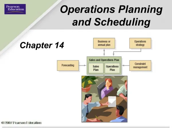
Sales and Operations Planning Resource Planning Demand Management Master Production Scheduling Detailed Capacity Planning Detailed Material Planning Material and Capacity Plans You are here Front end Engine Shop-Floor Systems Supplier Systems Back end
Example Job Processing Time Due 1 6 18 2 2 6 3 3 9 4 4 11 5 5 8 What order should we do them in?
Job Characteristics • Arrival pattern: static or dynamic • Number and variety of machines • We will assume they are all identical • Number of workers • Flow patterns of jobs: • all follow same, or many different • Evaluation of alternative rules
Objectives Many possible objectives: • Meet due dates • Minimize WIP • Minimize average flow time through • High worker/machine utilization • Reduce setup times • Minimize production and worker costs
Terminology Flow shop: all jobs use M machines in same order Job shop: jobs use different sequences Parallel vs. sequential processing Flow time: from start of first job until completion of job I Makespan: start of first to finish of last Tardiness: >= 0 Lateness: can be <0 or >0
Sequencing Rules First-come, first-served (FCFS) order they entered the shop Shortest Processing Time (SPT) longest job done last Earliest Due Date (EDD) job with last due date goes last Critical Ratio (CR) - processing time / time until due, smallest ratio goes first
Other rules • R - Random • LWR - Least Work Remaining • FOR - Fewest Operations Remaining • ST - Slack Time • ST/O-Slack Time per Operation • NQ-Next Queue – choose job that is going next to the machine with smallest queue • LSU - Least Setup
Performance Quantities of interest Li Lateness of i: can be +/- Ti Tardiness of i: always >= 0 Ei Earliness of i Tmax Maximum tardiness
Example: FCFS Job Time Done Due Tardy 1 6 6 18 0 2 2 8 6 2 3 3 11 9 2 4 4 15 11 4 5 5 20 8 12 Total 50 20 Mean flow time = 50 / 5 = 10.0 Average tardiness = 20 / 5 = 4.0 Number of tardy jobs = 4 Max. Tardy 12
Example: SPT Job Time Done Due Tardy 2 2 2 6 0 3 3 5 9 0 4 4 9 11 0 5 5 14 8 6 1 6 20 18 2 Total 50 8 Mean flow time = 50 / 5 = 10.0 Average tardiness = 8 / 5 = 1.6 Number tardy = 2 Max Tardy 6
Example: EDD Job Time Done Due Tardy 2 2 2 6 0 5 5 7 8 0 3 3 10 9 1 4 4 14 11 3 1 6 20 18 2 Total 51 6 Mean flow time = 51 / 5 = 10.2 Average tardiness = 6 / 5 = 1.2 Number tardy = 3 Max Tardy = 3
Critical Ratio Critical ratio: • looks at time remaining between current time and due date • considers processing time as a percentage of remaining time • CR = 1.0 means just enough time • CR > 1 .0 more than enough time • CR < 1.0 not enough time
Example: Critical Ratio • T = 0 Process Critical JobTimeDueRatio 1 6 18 3.0 2 2 6 3.0 3 3 9 3.0 4 4 11 2.75 5 5 8 1.6 Job 5 is done first.
Example: Critical Ratio • T = 5 Process Due - Critical JobTimeCurrentRatio 1 6 13 2.17 2 2 1 0.5 3 3 4 1.33 4 4 6 1.5 Job 2 is done second.
Example: Critical Ratio • T = 7 Process Due - Critical JobTimeCurrentRatio 1 6 11 1.84 3 3 2 0.67 4 4 4 1.0 Job 3 is done third.
Example: Critical Ratio • T = 10 Process Due - Critical JobTimeCurrentRatio 1 6 8 1.84 4 4 1 0.25 Job 4 is done fourth, and job 1 is last.
Critical Ratio Solution Job Time Done Due Tardy 5 5 5 8 0 2 2 7 6 1 3 3 10 9 1 4 4 14 11 3 1 6 20 18 2 Total 56 7 Mean flow time = 56 / 5 = 11.2 Average tardiness = 7 / 5 = 1.4 Number tardy = 4 Max Tardy 3
Summary Average Number Max Method Flow Tardiness tardy Tardy FCFS 10.0 4.0 4 12 SPT 10.0 1.6 2 6 EDD 10.0 1.2 3 3 CR 11.2 1.4 4 3
Minimizing Average Lateness • Mean flow time minimized by SPT • For single-machine scheduling, minimizing the following is equivalent: • Mean flow time • Mean waiting time • Mean lateness
Minimize Max Lateness • Earliest Due Date (EDD) minimizes maximum lateness
Minimizing Number of Tardy Jobs Moore’s Algorithm: 1. Start with EDD solution 2. Find first tardy job, i. None? Goto 4 3. Reject longest job in 1- i. Goto 2. 4. Form schedule by doing rejected jobs after scheduled jobs. • Rejects can be in any order, because they will all be late.
Moore’s Example Start with EDD schedule Job Time Done Due Tardy 2 2 2 6 0 5 5 7 8 0 3 3 10 9 1 4 4 14 11 3 1 6 20 18 2 Job 3 is first late job. Job 2 is longest of jobs 2,5,3.
Moore’s Example Job Time Done Due Tardy 2 2 2 6 0 3 3 5 9 0 4 4 9 11 0 1 6 15 18 0 5 5 20 8 12 Average Flow = 51 / 5 = 10.2 Average tardiness = 12 / 5 = 2.4 Number tardy = 1 Max. Tardy = 12
Summary 2 Average Number Max Method Flow Tardiness tardy Tardy FCFS 10.0 4.0 4 12 SPT 10.0 1.6 2 6 EDD 10.0 1.2 3 3 CR 11.2 1.4 4 3 Moore’s 10.2 2.4 1 12
Multiple Machines • N jobs on M machines: • (N!)Mpossible sequences. • For 5 jobs and 5 machines = 25 billion • Complete enumeration is not the way
Multiple Machines • 2 jobs, 2 machines. Job M1 M2 I 4 1 J 1 4 Four possible sequences:
Multiple Machines • 2 jobs, 2 machines. Job M1 M2 M1 M2 I 4 1 1 I J I J J 1 4 2 I J J I 3 J I J I Four possible 4 J I I J sequences:
J J J J J J J J Two Machines Makespan Sequence I IJ IJ IJ JI JI IJ JI JI 9 10 10 6 I I I I I I I
Two Machines • Permutation schedules: IJ IJ, JI JI • Jobs processed same sequence on both • For N jobs on two machines, there will always be an optimal permutation schedule.
2 Machines, N Jobs(Johnson’s Algorithm) Ai = processing time of job I on machine A Bi = processing time of job I on machine B 1. List Ai and Bi in two columns 2. Find smallest in two columns. If it is in A, schedule it next, if it’s in B, then last. 3. Continue until all jobs scheduled.
Johnson Example JobA B 1 5 2 2 1 6 3 9 7 4 3 8 5 10 4 Seq: 2, , , , 1. Job 2 is smallest, so it goes first.
Johnson Example JobA B 1 5 2 2 1 6 3 9 7 4 3 8 5 10 4 Seq: 2, , , , 1 1. Job 2 goes first. 2. Job 1 is next smallest, in B, so goes last.
Johnson Example JobA B 1 5 2 2 1 6 3 9 7 4 3 8 5 10 4 Seq: 2, 4 , , , 1 1. Job 2 goes first. 2. Job 1 goes last. 3. Job 4 is smallest, in A column, so it goes next.
Johnson Example JobA B 1 5 2 2 1 6 3 9 7 4 3 8 5 10 4 Seq: 2, 4, , 5, 1 1. Job 2 goes first. 2. Job 1 goes last. 3. Job 4 goes next. 4. Job 5 smallest in B, comes next to last.
Johnson Example JobA B 1 5 2 2 1 6 3 9 7 4 3 8 5 10 4 Seq: 2, 4, 3, 5, 1 1. Job 2 goes first. 2. Job 1 goes last. 3. Job 4 goes next. 4. Job 5 next to last. 5. Job 3 comes next.
Conclusions • Single machine scheduling: • FCFS, SPT, EDD, CR, Moore’s Algorithm • Two machines: • Johnson’s Algorithm • Performance: • Avg Lateness, Max Tardy, Avg Tardy, Number of jobs Tardy
Scheduling Days Off • Compute no. people needed each day. • Find the smallest two consecutive days • Highest number in the pair is <= highest number in any other pair • Those two days will be the first worker’s days off • Subtract one from the days the first worker wasn’t scheduled • Repeat
Example – Workers needed each day M T W Th F Sa Su 4 3 4 2 3 1 2
Example M T W Th F Sa Su #1 4 3 4 2 3 1 2 #2 3 2 3 1 2 1 2 #3 2 1 2 0 1 1 2 #4 1 0 1 0 1 0 1 #5 0 0 0 0 1 0 0
Example - Retry M T W Th F Sa Su #1 4 3 4 2 3 1 2 #2 3 2 3 1 2 1 2 #3 2 1 2 0 2 1 1 #4 1 0 1 0 1 1 1 #5 0 0 1 0 0 0 0
Example – 4 days M T W Th F Sa Su #1 4 3 4 2 3 1 2 #2 3 2 3 1 2 1 2 #3 2 1 2 0 1 1 2 #4 1 0 1 0 1 0 1 Do you want to work the #4 schedule?
Scheduling Daily Work Times • Different # people needed in different areas at different times
Scheduling Hourly Times • When should people start shifts? • “First Hour” principle: • For first hour, assign # people needed that hour • Each additional hour, add more if needed • When shift ends, add more, only if needed
Hourly Work Times 10 11 12 1 2 3 4 5 6 7 8 9 Need 4 6 8 8 6 4 4 6 8 10 10 6 Start 4 2 2 0 0 0 0 0 4 4 2 0 On 4 6 8 8 8 8 8 8 8 10 10 10
Production vs. Transfer batch sizes p. 552 Lot Sizes all 1,000 Production Lot Size = 1,000 Transfer Batch Size = 100 Production Lot Size = 200 Transfer Batch Size = 100 Production Lot Size = 500
HW, p. 567 – Due 12/9 • DQ: 4 • Problems: 1,2,3,4,5