Download
1 / 30
300 likes | 409 Vues
Explore complexities of railroad planning & operations, including traffic demand estimation, blocking plans, & train scheduling. Learn about capacity, OD demand, and freight estimation methods.

E N D
Operations Research Models for Railroad Routing and Scheduling Problems Xuesong Zhou University of Utah zhou@eng.utah.edu
Outline • Background on railroad planning and operations • Traffic OD demand estimation problem • Railroad blocking problem and line planning problem • Train timetabling and dispatching problems • Research directions
Railroad Network Capacity • Line capacity • Single or double-track -> meet-pass plans • Signal control type -> minimal headways • Locomotive power -> speed, acceleration/deceleration time loss • Train schedules -> overall throughput • Node capacity (yards, terminals / sidings) • Track configuration (# of tracks, track lengths, switcher engines) • Locomotive power-> car processing time • Yard make-up plans, terminal operating plans -> overall throughput
OD Demand ->Routes-> Blocks-> Trains • Origin destination (OD) traffic demand • Commodities, commercial unit traffic groups, car equipment requirement • Route plan • Single route or multiple routes for each OD pair • Blocking plan • Block origin, block destination, commodities, final destinations • Standard, local, unit • Make-up plan • Block-to-train assignment • Train schedule • Arrival and departure times, station dwell times • Block assignment and order • Local/express, freight/passenger • Trip plan • Distance, transit time • Block sequence and intermediate classification yards
How to Estimate Freight OD Demand Matrix? • Input-output models (Leontieff, 1936) • Spatial interaction models • Gravity models • Direct demand models ( functions of socio-economic characteristics) • Trip-based spatial interaction models • Trip generation, trip distribution, trip assignment • Commodity-based spatial interaction models • Commodity generation, commodity distribution, mode split, trip assignment • Origin destination demand estimation based on link counts
Traffic OD Demand Estimation Problem • Given • Network • Network zone structure • Socio-economic data and interview samples • Historical demand information • Link counts cl • Find • Freight/ Passenger OD matrix di,j where i,j = zone index l = link index pl,i,j= link flow proportion, i.e. fraction of traffic demand flow from OD pair( i,j) contributing to the flow on link l e= measurement noise • Measurement Equations • cl=Σi,j,tpl, i,j× di,j+
Freight OD Demand Estimation Models • Linear programming model with multiple vehicle classes • List and Turnquist, 1994 • Entropy model with given link flow proportion matrix • Jornsten and Wallace,1993 • Linear programming model with simple route choice model • Sherali et al.1994 • Bi-level model for multimode multi-product freight transportation • Crainic et al. 2001 • Upper level: • Lower level: Pl,i,j = System optimum traffic assignment (di,j) • Holguin-Veras, et al. 2004 Lower level: market equilibrium
Railroad Blocking Problem • Given • Network G=(N,A) • Freight shipments with different origins/destinations • Find • Blocking plan that can route all shipments over the network • Which blocks to build at each yard • Sequences of blocks to deliver each shipment • Constraints • Node capacity (yard processing volume) • Maximal # of outbound arcs (blocks) for each node • # of classification tracks at a yard • Objective Functions • Minimize total travel distance • Minimize intermediate handlings cost • Minimize delay cost • Network representation • Classification yards: nodes->arcs • Candidate blocks: express arcs that bypass yards
Network Design Formulation Linear cost, multi-commodity capacitated network design problem • Minimize (i,j)A fijyij + kK (i,j) cij xkij subject to: • Flow conservation constraint (i,j)O(i) xkij - (j,i)I(i)xkij = dki for all i N for all k K • Yard capacity constraint kK xkij≤ uijyij for all (i, j) A • Limit on # of blocks that may be built at each yard (i,j)O(i) yij≤ vi for all i N where k = commodity/product index (origin, destination, traffic class) yij = 0-1 design variable for opening block (i,j) or not xkij= amount of flow of commodity k using block (i,j) fij= fixed cost of opening block (i,j) cij= transportation cost of moving per unit of commodity on arc (i,j) dki=demand of commodity k at node i uij=capacity of link (i,j)
Blocking Plan Optimization Models (I) • Bodin, Golden and Schuster (1980) • Arc-based multi-commodity flow formulation • No freight priorities • Assad (1983) • Dynamic programming formulation for a rail line • Crainic, Ferland and Bousseau (1984) • Consider blocking, train routing, and block-to-train assignment • Nonlinear objective with queuing-based delay estimate • Column generation to introduce attractive block and train • Van Dyke (1986, 1999) • Improve existing blocking plan • Augmented shortest path • Keaton (1989,1992) • Consider blocking, train routing and block-to-train assignment • Dual adjustment procedure based on Lagrangian relaxation
Blocking Plan Optimization Models (II) • Huntley (1995) • Meta-heuristic solution algorithms • Newton (1996), Newton et al. (1998), Barnhart et al. (2000) • Path-based multi-commodity flow formulation • Branch-and-price, branch-and-cut • Dual-based Lagrangian relaxation with sub-gradient optimization • Ahuja, et al. (2004) • Very Large-Scale Neighborhood (VLSN) search • Start with feasible solutions • Improve/re-optimize solutions for each node (yard) • Multiple passes over the nodes
Line Planning • Given • Network G=(N,A) • Traffic demand with different origins/destinations • Find • Routes, frequencies, and stop schedules • Constraints • Train capacity • Objective Functions • Minimize total travel time • Minimize total number of train units
Frequency Service Network Design Formulation • Minimize sS fsys + kK sS c(xks, ys) subject to: • Flow conservation constraint sSσ(k,s)xk = dk for all k K • Service capacity constraint kK xks≤ usys for all s S where k = index for commodity (origin, destination, traffic class) s = index for service that defines train origin, destination, route, intermediary terminals with stops ys = frequency of service s (integer variable) xks= amount of flow of commodity k using service s fs= fixed cost of operating one train for service s c(xks, ys)= transportation cost/delay of moving commodity k by using service s σ(k,s) = commodity-service indicator, 1: commodity k can use service s, 0 otherwise dk=demand of commodity k us= capacity of one train for service s
Frequency Service Network Design Models • Crainic and Rousseau (1996) • Network design formulation • Decomposition solution approach • Column generation to find attractive itineraries • Bussieck and Zimmermann (1997), Bussieck (1998) • Line planning problem • Passenger rail network with periodic schedules • Maximize direct travelers • Mixed integer programming formulation • Branch-and-cut solution method to use utilize polyhedral structure • Goossens, Hoesel and Kroon (2004) • Branch-and-cut with valid inequalities
Dynamic Service Network Design • Time-space network • Physical network represented at each period • Service arcs: represent each possible departure of each service • Waiting/holding (inventory) arcs: connect two nodes representing the same terminals in consecutive periods • Decision variables • 0-1 variables: whether or not the service leaves at the specified time • Continuous path flow through the service network
Dynamic Service Network Design Models • Morlok and Peterson (1970) • Integrate blocking, train formulation, and train scheduling • Large mixed integer programming formulation • Haghani (1989) • Integrate train make-up, routing and empty car distribution • Empty and loaded car flows, engine flows • Gorman (1998) • Consider operating plan that minimizes operating costs, meets customer’s service requirements • Generate candidate train schedules, and then evaluate economic, service, and operational performance
Train Timetabling and Dispatching Problem • Given • Line track configuration • Minimum segment and station headways • # of trains and their arrival times at origin stations • Find • Timetable: Arrival and departure times of each train at each station • Objectives • (Planning) Minimize the transit times and overall operational costs, performance and reliability • (Dispatching) Minimize the deviation between actual schedules and planned schedule
Resource Constrained Project Scheduling Formulation • Project i = train i with a sequence of K activities • Activity (i, k) = train i traveling section k • Renewable resources k: entering times and leaving times of station k • Mode m = stop-stop, stop-pass, pass-stop, pass-pass • Processing time pt(i,k,m) = traveling time with acceleration and deceleration time losses • Precedence constraint: minimum headway constraints for two consecutive activities at the same station
Integer Programming Formulation or • Minimize • Departure time constraint • Dwell time constraint • Travel time on sections • Minimum headway constraint (N× (N-1) ×K× 4 constraints)
Branch-and-Bound Solution Algorithm (I) • Step 1: (Initialization) Create a new node, in which contains the first task of all trains. Set the departure time for this train and insert this node into active node list (L). • Step 2: (Node Selection) Select an active node from L according to a given node selection rule. • Step 3: (Stopping criterion) If all of active nodes in L have been visited, then terminate. • Step 4: (Conflict set construction) Update the schedulable set in the selected node . Scan all the tasks this set , and find a task t(i,j) with the minimal end time and all the tasks that invalidate the headway constraint. Insert these tasks and task t(i,j) into the current conflict set.
Branch-and-Bound Solution Algorithm (II) • Step 5: (Active schedule generation) For each task in the conflict set, create a new active node and insert it into L. Fix a task in the conflict set and right-shift the start time of the other conflict tasks according to the headway requirement with respect to the fixed task. • Step 6: (Lower bound) Compute the lower bound , If LB>Z, fathom this node, go to step 2. If conflict set is empty, this indicates all the tasks have been finished and the related schedule is feasible. Furthermore, if the current schedule is a feasible one with a smaller objective function value Z’ , then update Z=Z’. • Step 7: (Dominance rule) Compare the current schedule with the other schedules at visited nodes, if the dominance conditions are satisfied, then dominated node is disabled, its associated successors will not be completed. Go to Step 2.
Illustration of Dominance Rules Decision point • Main Idea: • Cut dominated partial schedule at early as possible • Conditions for node a dominating node b • Same set of finished trains • Z(a) < Z(b) for finished trains • The starting time for each unfinished activity in node a is no later than the counterpart in node b for each feasible mode
Exact Solution Algorithms • Szpigel (1973) • Job-shop scheduling formulation • Branch-and-bound solution algorithm • Chen and Harker (1990); Jovanovic and Harker (1991) • Considers reliability (on-time performance) of planed schedules under random travel times • Higgins et al. (1995); Higgins and Kozan (1998) • Inexact lower bound that estimates possible delay • Multi-criteria scheduling framework that considers fuel costs for locomotives, labor costs for crews • Brannlund et al. (1998) • Lagrangian lower bound that relaxes the segment capacity • Peeters and Kroon (2001); Kroon and Peeters (2003) • Cyclic railway timetabling • Zhou (2005) • Exact lower bound for estimating possible delay • Dominance rules
Heuristic Solution Algorithms • Simple priority rule-based methods (used in simulation systems) • Minimal-delay criterion (MinDelay); Shortest departure time rule (SDT) • First-in-first-out rule (FIFO); Shortest processing time rule (SPT) • Improved priority rule-based methods used in the train scheduling field • Look-ahead method (Sahin, 1999) • Evaluation horizon only covers all the conflict trains at the current node • Global priority rule (Higgins et al., 1995) • Find a feasible solution by applying a simple local rule successively • Use the corresponding objective function value as the estimation value • Backtracking method (Adenso-Diaz el at., 1999) • Use a local rule to find a feasible schedule • Backtrack the search tree until k nodes have been examined • Beam search (Zhou, 2005) • Beam search algorithm uses a certain evaluation rule to select the α-best nodes to be computed at next level Look-ahead method Global priority rule • Meta-heuristics (Higgins, et al. 1997)
Train Routing Problem at Terminals • Given • Track configuration ( track lengths, switcher engines ) • Signal configuration • Inflow/Outflow (arrival and departure times of trains) • Find • Train paths through a terminal • Choke points • System performance of a rail facility under a variety of conditions
Train Routing through Terminals • Switch Grouping • Train Paths • Train type I: switch groups a, b, d • Train type II: switch groups c, d, e • Train type III: switch groups f, g, h • Carey and Lockwood (1995); Carey (1994) • Mixed integer programming formulation • Heuristic solution algorithm • Zwaneveld, Kroon, Hoesel (2001); Kroon, Romeijn, Zwaneveld (1997) • Complexity issues • Node packing model
North American Railroad Network 5 major US railroads after years of consolidations: CSX, UP, CR, NS, BNSF
Research Directions • Robust schedule design • Executable vs. recoverable, from planning to real-time decision • Improve freight railroad service reliability • Disruption management under real time information • Service networks (blocking and line planning) • Train dispatching • Rail network and terminal capacity recovery plan • Locomotive and crew recovery plan • Integrated pricing and demand management model • Long term and short term pricing schemes and cost structures • Separation of track from traction in Europe • Impact on traffic demand and operating plans (train schedule, fleet sizing and repositioning) • Shipper logistics modeling • Demand estimation and prediction model