Models for Epidemic Routing
640 likes | 671 Vues
Learn about Markovian and Fluid models for optimizing message delay and mobility impact on ad hoc networks. Explore epidemic routing scenarios and performance metrics with case examples. Enhance your routing strategies today!

Models for Epidemic Routing
E N D
Presentation Transcript
Models for Epidemic Routing Giovanni Neglia INRIA – EPI Maestro 20 January 2010 Some slides are based on presentations from R. Groenevelt (Accenture Technology Labs) and M. Ibrahim (previous Maestro PhD student)
Outline • Introduction on Intermittently Connected Networks (or Delay/Disruption Tolerant Networks) • Markovian models • Message Delay in Mobile Ad Hoc Networks, R. Groenevelt, G. Koole, and P. Nain, Performance, Juan-les-Pins, October 2005 • Impact of Mobility on the Performance of Relaying in Ad Hoc Networks, A. Al-Hanbali, A.A. Kherani, R. Groenevelt, P. Nain, and E. Altman, IEEE Infocom 2006, Barcelona, April 2006 • Fluid models • Performance Modeling of Epidemic Routing, X. Zhang, G. Neglia, J. Kurose, D. Towsley, Elsevier Computer Networks, Volume 51, Issue 10, July 2007, Pages 2867-2891
Intermittently Connected Networks • mobile wireless networks • no path at a given time instant between two nodes • because of power contraint, fast mobility dynamics • maintain capacity, when number of nodes (N) diverges • Fixed wireless networks: C = Θ(sqrt(1/N)) [Gupta99] • Mobile wireless networks: C = Θ(1), [Grossglauser01] • a really challenging network scenario • No traditional protocol works V2 V3 B V1 C A
Some examples Inter-planetary backbone DieselNet, bus network DakNet, Internet to rural area ZebraNet, Mobile sensor networks • Network for disaster relief team • Military battle-field network • …
Terminology and Focus • Why delay tolerant? • support delay insensitive app: email, web surfing, etc. • Why disruption tolerant? • almost no infrastructure, difficult to attack • post 9/11 syndrome • In this lecture we only consider case where there is no information about future meetings • how to route?
Epidemic Routing V2 V3 B V1 C A • Message as a disease, carried around and transmitted
Epidemic Routing V2 V3 B V1 C A • Message as a disease, carried around and transmitted • Store, Carry and Forward paradigm
Epidemic Routing V1 A V3 C B V2 • Message as a disease, carried around and transmitted • How many copies? • 1 copy ⇨ max throughput, very high delay • More ⇨ reduce delay, increase resource consumption (energy, buffer, bandwidth) • Many heuristics proposed to constrain the infection • K-copies, probabilistic…
Standard Epidemic Routing t1 S 2 2 t2 3 3 4 4 5 5 D D TD Time
Epidemic Style Routing • Epidemic Routing [Vahdat&Becker00] • Propagation of a pkt -> Disease Spread • achieve min. delay, at the cost of transm. power, storage • trade-off delay for resources • K-hop forwarding, probabilistic forwarding, limited-time forwarding, spray and wait…
2-Hop Forwarding t0 S 2 2 3 3 4 5 5 D D TD At most 2 hop Time
Limited Time Forwarding t0 S 2 2 3 3 4 4 5 5 3 D Time
Epidemic Style Routing • Epidemic Routing [Vahdat&Becker00] • Propagation of a pkt -> Disease Spread • achieve min. delay, at the cost of transm. power, storage • trade-off delay for resources • K-hop forwarding, probabilistic forwarding, limited-time forwarding, spray and wait… • Recovery: deletion of obsolete copies after delivery to dest., e.g., • TIMERS: when time expires all the copies are erased • IMMUNE: dest. cures infected nodes • VACCINE: on pkt delivery, dest propagates anti-pkt through network
IMMUNE Recovery t0 S 2 2 3 3 4 4 5 5 D D TD 4 4 7 Time 8 8
VACCINE Recovery t0 S 2 2 3 3 4 4 5 5 D D TD 4 4 7 7 Time 8 8 2 2
Outline • Introduction on Intermittently Connected Networks (or Delay/Disruption Tolerant Networks) • Markovian models • the key to Markov model • Markovian analysis of epidemic routing • Fluid models
S 2 The setting we consider • N+1 nodes • moving independently in an finite area A • with a fixed transmission range r and no interference • 1 source, 1 destination • Performance metrics: • Delivery delay Td • Avg. num. of copies at delivery C • Avg. total num. of copies made G • Avg. buffer occupancy D 3 N
Standard random mobility models Random Waypoint model (RWP) Random Direction model (RD) X2 V2 T2, V2 X1 α2 V1 T1, V1 R α1 R • Directions (αi) are uniformly distributed(0, 2π) • Speeds (Vi) are uniformly distributed (Vmin,Vmax) • Travel times (Ti) are exponentially /generally distributed • Next positions (Xi)s are uniformly distributed • Speeds (Vi)s are uniformly distributed(Vmin,Vmax)
The key to Markov model • [Groenevelt05] • if nodes move according to standard random mobility model (random waypoint, random direction) with average relative speed E[V*], • and if Nr2 is small in comparison to A • pairwise meeting processes are almost independent Poisson processes with rate: w: mobility specific constant
Intuitive explanation Exponential distribution finds its roots in the independence assumptions of each mobility model: • Nodes move independently of each other • Random waypoint: future locations of a node are independent of past locations of that node. • Random direction: future speeds and directions of a node are independent of past speeds and directions of that node. There is some probability q that two nodes will meet before the next change of direction. At the next change of direction the process repeats itself, almost independently.
Why “almost”? • pairwise meeting processes are almost independent Poisson processes with rate: • inter-meeting times are not exponential • if N1 and N2 have met in the near past they are more likely to meet (they are close to each other) • the more the bigger it is r2 in comparison to A • meeting processes are not independent • if in [t,t+τ] N1 meets N2 and N2 meets N3, it is more likely that N1 meets N3 in the same interval • the more the bigger it is r2 in comparison to A • moreover if Nr2 is comparable with A (dense network) a lot of meeting happen at the same time. w: mobility specific constant
Examples Nodes move on a square of size 4x4 km2 (L=4 km) Different transmission radii (R=50,100,250 m) Random waypoint and random direction: no pause time [vmin,vmax]=[4,10] km/hour Random direction: travel time ~ exp(4)
The derivation of λ Assume a node in position (x1,y1) moves in a straight line with speed V1. Position of the other node comes from steady-state distribution with pdf π(x,y). Look at the area A covered in Δt time: V* V*Δt
The derivation of λ Probability that nodes meet given by For small r the points in π(x,y) in A can be approximated by π(x1,y1) to give Unconditioning on (x1,y1) gives
The derivation of λ Proposition: Let r<<L. The inter-meeting time for the random direction and the random waypoint mobility models is approximately exponentially distributed with parameter Here E[V*]is the average relative speed between two nodes and is the pdf in the point (x,y). 9
The derivation of λ Proposition: Let r<<L. The inter-meeting time for the random direction and the random waypoint mobility models is approximately exponentially distributed with parameter Here E[V*] is the average relative speed between two nodes and ω≈ 1.3683 is the Waypoint constant. If speeds of the nodes are constant and equal to v, then
Summary up to now • First steps of this research • a good intuition • some simulations validating the intuition for a reasonable range of parameters • What could have been done more • prove that the results is asymptotically (r->0) true “in some sense” • What can be built on top of this? • Markovian models for routing in DTNs
2-hop routing Model the number of occurrences of the message as an absorbing Markov chain: • State i{1,…,N} represents the number of occurrences of the message in the network. • State A represents the destination node receiving (a copy of) the message.
Epidemic routing Model the number of occurrences of the message as an absorbing Markov chain: • State i{1,…,N} represents the number of occurrences of the message in the network. • State A represents the destination node receiving (a copy of) the message.
Message delay Proposition: The Laplace transform of the message delay under the two-hop multicopy protocol is: and
Message delay Proposition: The Laplace transform of the message delay under epidemic routing is: and
Expected message delay Corollary: The expected message delay under the two-hop multicopy protocol is and under the epidemic routing is Where γ ≈ 0.57721 is Euler’s constant.
Relative performance The relative performance of the two relay protocols: and Note that these are independent of λ!
Some remarks • These expressions hold for any mobility model which has exponential meeting times. • Two mobility models which give the same λ also have the same message delay for both relay protocols! (mobility pattern is “hidden” in λ) • Mean message delay scales with mean first-meeting times. • λ depends on: - mobility pattern - surface area - transmission radius
Example: two-hop multicopy Distribution of the number of copies (R=50,100,250m):
Example: two-hop multicopy Distribution of the number of copies (R=50,100,250m):
Example: two-hop multicopy Distribution of the number of copies (R=50,100,250m):
Outline • Introduction on Intermittently Connected Networks (or Delay/Disruption Tolerant Networks) • Markovian models • the key to Markov model • Markovian analysis of epidemic routing • Fluid models
1 2 3 N-2 N N-1 D Why a fluid approach? • [Groenevelt05] • Markov models can be developed • States: nI =1,…, N: num. of infected nodes, different from destination; D: packet delivered to the destination • Transient analysis to derive delay, copies made by delivery; hard to obtain closed form, specially for more complex schemes Infection rate: Delivery rate:
Modeling Works: Small and Haas • Mobicom 2003 [small03] • ODE introduced in a naive way for simple epidemic scheme • N is the total number of nodes, • I the total number of infected nodes • λ is the average pairwise meeting rate • Average pair-wise meeting rate obtained from simulations • TON 2006 [haas06] • consider a Markov Chain with N-1 different meeting rates depending on the number of infected nodes (obtained from simulations) • Numerical solution complexity increases with N
Our contribution (1/3) • A unified ODE framework... • limiting process of Markov processes as N increases [Kurtz 1970]