Introduction to Robotics

1. Introduction to Robotics Dept. of Computer Science Technion Winter Semester, 2004-5

2. I2R Information Sheet • Instructor: Hector Rotstein • Phone: 054-2151054. Evenings only! • Office hours: Mo: 17:30-18:30 Fri: 11:30 - 12:30 (appointment only) • E-mail: hector@ee.technion.ac.il

3. I2R Information Sheet

4. Bibliography • John Craig, “Introduction to robotics,” Addison Wesley. • G. Dudek and M. Jenkin, “Computational Principles of Mobile Robotics,” Cambridge University Press. • Handouts

5. Course Objectives At the end of this course, you should be able to: • Describe and analyze rigid motion. • Write down manipulator kinematics and operate with the resulting equations • Solve simple inverse kinematics problems. • Select sensors for performing robotic tasks • Use sensors to compute robotics localization

6. Syllabus • A brief history of robotics. Coordinates and Coordinates Inversion. Trajectory planning. Sensors. Actuators and control. Why robotics? • Basic Kinematics. Introduction. Reference frames. Translation. Rotation. Rigid body motion. Velocity and acceleration for General Rigid Motion. Relative motion. Homogeneous coordinates. • Robot Kinematics. Forward kinematics. Link description and connection. Manipulator kinematics. The workspace.

7. Syllabus (cont.) • Inverse Kinematics. Introduction. Solvability. Inverse Kinematics. Examples. Repeatability and accuracy. • Basic Dynamics and Control. Introduction. Definitions and notation. Laws of Motion. Robot control. • Trajectory generation. Introduction. General considerations. Path generation. • Introduction to mobile robots. Mobile Robots hw. • Sensing and localization

8. Policies and Grades • There will be six homework assignments, one mid-term and one final. • Tests are open book. The homeworks will count 4% each towards the final grade, the test 40% and the final 36%. • The worst homework will be given 20% of the normal weight, while the best will be given 180% of the normal weight.

9. Policies and Grades (cont.) • Collaboration in the sense of discussions is allowed. You should write final solutions and understand them fully. Violation of this norm will be considered cheating, and will be taken into account accordingly. • Can work alone or in teams of 2 • You can also consult additional books and references but not copy from them.

10. Policies and Grades (cont.) • Required homework will be due before the beginning of practice, at the course mailbox. • Late homework will be accepted up to one week after the due date, will receive a maximum grade of 80% and loose 10% for each delay day after the first one. However, bonus problems must be handed in on their due date.

11. Robot Examples

12. The Three Laws of Robotics • A robot may not injure a human being, or, through inaction, allow a human being to come to harm. • A robot must obey the orders given it by human beings except where such orders would conflict with the First Law. • A robot must protect its own existence as long as such protection does not conflict with the First or Second Law. Zeroth law: A robot may not injure humanity, or, through inaction, allow humanity to come to harm

13. Robot Demos

14. A Brief History of Robotics • The word robot introduced by Czech playwright Karel Capek: robots are machines which resemble people but work tirelessly. • His view is still to be fulfill! Best soccer player ever Best robot player ever

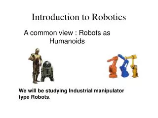
15. A Brief History of Robotics II • Definition: a robot is a software-controllable mechanical device that uses sensors to guide one or more end-effectors through programmed motions in a workspace in order to manipulate physical objects. • Today’s robots are not androids built to impersonate humans. • Manipulators are anthropomorphic in the sense that they are patterned after the human arm. • Industrial robots: robotic arms or manipulators

16. History of Robotics (cont.) • Early work at end of WWII for handling radioactive materials: Teleoperation. • Computer numerically controlled machine tools for low-volume, high-performance AC parts • Unimation (61): built first robot in a GM plant. The machine is programmable. • Robots were then improved with sensing: force sensing, rudimentary vision.

17. History of Robotics (cont.) • Two famous robots: • Puma. (Programmable Universal Machine for Assembly). ‘78. • SCARA. (Selective Compliant Articulated Robot Assembly). ‘79. • In the ‘80 efforts to improve performance: feedback control + redesign. Research dedicated to basic topics. Arms got flexible. • ‘90: modifiable robots for assembly. Mobile autonomous robots. Vision controlled robots. Walking robots.

18. Robot Classification Robotic manipulator: a collection of links inter- connected by flexible joints. At the end of the robot there is a tool or end-effector. • Drive Technology. Which source of power drives the joints of the robot. • Work-envelope geometries. Points in space which can be reached by the end-effector. • Motion control method. Either point-to-point or continuous path

19. The Course at a Glimpse: Kinematics F(robot variables) = world coordinates x = x(1,, n) y = y(1,, n) z = z(1,, n) • In a “cascade” robot, Kinematics is a single-valued mapping. • “Easy” to compute.

20. r  workspace Kinematics: Example 1= , 2=r 1 r  4.5 0   50o x = r cos  y = r sin 

21. Inverse Kinematics • G(world coordinates) = robot variables 1 = 1(x,y,z)  N= N(x,y,z) • The inverse problem has a lot of geometrical difficulties • inversion may not be unique!

22. 2 1 Inverse Kinematics: Example Make unique by constraining angles

23. Trajectory Planning • Get from (xo, yo, zo) to (xf, yf, zf) • In robot coordinates: o  f • Planning in robot coordinates is easier, but we loose visualization. • Additional constraints may be desirable: • smoothness • dynamic limitations • obstacles