Unsupervised Machine Learning Algorithms
Unsupervised Machine Learning Algorithms. Unsupervised Machine Learning Algorithms. Unsupervised learning is typically used in finding special relationships within data set No training examples used in this process The system is given a set of data to find the patterns and correlations therein

Unsupervised Machine Learning Algorithms
E N D
Presentation Transcript
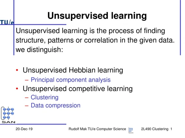
Unsupervised Machine Learning Algorithms • Unsupervised learning is typically used in finding special relationships within data set • No training examples used in this process • The system is given a set of data to find the patterns and correlations therein • Attempt to describe hidden structures or properties in the entire input data set • The examples given are unlabeled • No error or reward signal to evaluate a potential solution • This distinguishes unsupervised learning from supervised learning and reinforcement learning • The unsupervised approach is related to two fundamental capabilities
Unsupervised Machine Learning Algorithms (cont.) • The density estimation in input data statistics • The ability to summarize and explain key data features • Unsupervised machine learning demands more skill • On data mining, data structuring, data preprocessing, feature extraction and pattern recognition • Without the help of labeled samples • Must sort out the unstructured data • To obtain the associations among data items, cluster data with similarity, reduce the dimension of the feature space, or change the representation format to enable visualization, etc
Unsupervised Machine Learning Algorithms (cont.) • Many machine learning methods applied in unsupervised learning • Based on data-mining methods to preprocess the unlabeled data • Some reported ML algorithms that operate without supervision • Including clustering methods, association analysis, dimension reduction, and artificial neural networks
Association Rule Learning • Association rule learning generates inference rules • Used to discover useful associations in large multidimensional data sets • Best explain observed relationships between variables in the data • These association patterns are often exploited by enterprises or large organizations • e.g., Association rules are generated from input data to identify close-knit groups of friends in a social network database • e.g., A priori principle and association rules
Association Analysis and A priori Principle • Association analysis is also known as association mining • Refers to finding frequent patterns, associations, correlation or causal structures • Exist in sets of projects and collection of objects in the transaction data, relational data or other information carriers • A way to find out the interesting association hidden in large datasets • The discovered links are expressed in association rules: X → Y • X and Y are data objects or patterns • The rule indicates a strong connection between the X and Y
Association Analysis and A priori Principle (cont.) • Shopping basket data of some customers • Through observation, some shoppers who order diapers also buy milk • A strong connection between diapers and milk sales • i.e., The association rule: {diapers → milk} • Each line corresponds to a transaction tj and an order ij
Association Analysis and A priori Principle (cont.) • I = {i1, i2,⋯, id} is a collection of all items in the shopping basket data • T = {t1, t2,⋯, tN} is a collection of all transactions • The set of items included in each transaction tj is a subset of I • In an association analysis • A set of items is defined as a collection of one or more items • If an itemset contains k items, it is called a k-itemset • e.g., {cola, beer, bread, diapers} is 4-item set • An important attribute is the support count • Defined as the number of transactions that contain a specific itemset X:
Association Analysis and A priori Principle (cont.) • The notation |⋅| represents the cardinality of a set • e.g., In terms of the itemset {milk, beer, diapers}, its support count of {milk, beer, diapers} is 2 • Only two transactions contain the three items, i.e., BuyerID 1 and BuyerID 4 • The degree of support for the itemset X s(X) = σ(X)/N • N is the total number of transactions • Denotes the frequency of the fact that the itemset is contained in the dataset • The greater the degree of support, the greater the intensity of the itemset: s(X) minsup • minsup is the threshold value of support degree • To find all the itemsets with the support degree greater than or equal to minsup
Association Analysis and A priori Principle (cont.) • One assumption for the association rule • X → Y, X ∩ Y = ∅ • The confidence level for an association rule • Represents the strength of association rules • i.e., The frequency of the fact that Y appears in the transactions containing X • Also the frequency of the fact that the rule is reflected in the dataset • The greater the confidence level, the greater the intensity of the association rules: • minconf is the threshold value of confidence level • To find all the association rules with the confidence level greater than or equal to minconf
Association Analysis and A priori Principle (cont.) • The object of the association analysis • To find the association rule whose itemset’s support degree and confidence level are relatively large in a given transaction set • This process is defined as association rule discovery • Discover the association rules is the key problem • Usually to enumerate all possible rules • Impractical for a set with large number of transactions • For a dataset with d items, the total number of potential association rules is R = 3d - 2d+1 + 1 • Any item z may be included in X, or Y, or not both • Exclude those combinations with X or Y being empty • The above procedure will exclude the case of both X and Y being empty twice
Association Analysis and A priori Principle (cont.) • e.g., The dataset that contains 7 items has 1932 association rules • To better find out the association rules • Use the concept of frequent itemsets and strong rules • For itemset X and its subset Xi • The number of rules is 𝜎(X) ≤ 𝜎(Xi) • A transaction that contains a certain set of items must also contains the subset of this set • The frequent itemset is defined as a set of items that satisfy the minimum support count threshold • i.e., All its subsets are frequent sets of items • Strong rules are defined as the association rules • The confidence level is high in frequent items
Association Analysis and A priori Principle (cont.) • Two major subtasks to discover the association rules • To find out all frequent itemsets • Known as the generation of frequent sets • To find out all the strong rules • Known as the generation of strong rules • The frequent itemsets demand an algorithm to specify its generation procedure • If an itemset is frequent, all its subsets must also be frequent • Known as the A priori principle • If an itemset is infrequent, all of its supersets are infrequent
Association Analysis and A priori Principle (cont.) • Using this principle based on support count to prune the exponential set • Utilizes the anti-monotone trait of support degree • The support degree of an itemset can never exceed that of its subset • The specific steps of the generation of A priori frequent itemsets • This algorithm generates the frequent itemsets to mine the association rules • Uses pruning technique based on support degree to solve the exponential explosion problem • The key point is how to generate candidate itemsets Ck • Three methods to prune unnecessary itemsets
Association Analysis and A priori Principle (cont.) • The order of magnitude and brief descriptions of the three pruning methods • Using A priori Principle to Predict Price Rising in a Department Store • The price data of commercial goods during the first eight months of one year
Association Analysis and A priori Principle (cont.) • 1 to refer to a price increase and 0 for no increase • Used to analyze the price relations as to whether there is a link between a pair of goods • The frequent itemsets are generated • Set minsup to 0.6 • Fk-1 × F1method is used to generate k-candidate itemsets to determine frequent itemsets
Association Analysis and A priori Principle (cont.) • First, the support degree of candidate 1-itemsets can be calculated • According to the support degree 0.6, B, D and E can be pruned (0.6×8 = 4.8) • Thus obtaining frequent 1-itemsets {A}, {C} • Using the method Fk-1 × F1 can generate the candidate 2-itemsets: {A, C} • Calculate the support degree of candidate 2-itemsets: 𝜎({A, C}) = 5 • All the k-frequent itemsets are {A}, {C}, {A, C}
Association Rule Generation • Each of the frequent itemsets can satisfy the threshold of the support degree • Each k-frequent itemset can generate as many as 2k - 2 association rules • Every its subset except itself and the empty set can generate an association rule • e.g., If the itemset is {1, 2, 3}, a frequent 3-itemset, it can generate six rules • The number of rules generated by this approach is too large • Does not necessarily meet the requirements of the confidence threshold
Association Rule Generation (cont.) • Need the confidence measure to reduce the number of rules to achieve pruning • The rule pruning technique is based on the degree of confidence • If the two rules X′ → Y − X′, X → Y − X meet the requirement of X′ ⊂ X • For a set of items that have the inclusive relationship, 𝜎(X′) ≥ 𝜎(X) exists • The confidence level of the previous rule must not exceed the latter confidence level
Association Rule Generation (cont.) • If the rule X → Y − X does not satisfy the confidence threshold • The rules such as X′ → Y − X′ with X′ ⊂ X will not satisfy the confidence threshold • The algorithm of the generation of A priori rules is based on the above theorem • The algorithm uses a layer-by-layer method to generate association rules • Each layer corresponds to the number of items in the rules • Initially, all rules with high confidence are extracted from the itemsets with one item after the extraction • These rules are used to generate new candidate rules
Association Rule Generation (cont.) • Steps of the generation of A priori rules • Does not need to scan the dataset again • To calculate the confidence level of the candidate rules • Can use the support count of the generation of frequent items to determine the degree of confidence level for each rule • Physical Check-up to Link Symptoms to Diseases • A data collection of physical examinations • For fatty liver, obesity, high blood pressure, diabetes and kidney stones from a general hospital in Wuhan • 1 refers to suffering from the disease and 0 means no • To analyze if there is a link between the diseases
Association Rule Generation (cont.) • Often a relationship between different diseases • One disease can be derived from another • Can help doctors to improve diagnostic efficiency and reduce the rates of misdiagnosis • Utilizing correlation analysis, these data are used to analyze if there is a link between these diseases
Association Rule Generation (cont.) • To find out whether there is an association between the sample transactions • First need to determine all the frequent itemsets in the transaction dataset • Use the frequent item to generate association rules • Assume that the support and confidence thresholds are 0.4 and 0.6, respectively • a, b, c, d, e respectively refers to fatty liver, obesity, high blood pressure, diabetes and kidney stones • The process of the generation of frequent itemsets • Use the method Fk-1 × F1to generate k-candidate itemsets to determine frequent itemsets • Calculate the outcome of candidate 1-itemsets
Association Rule Generation (cont.) • According to the by support threshold 0.4, d and e can be pruned (0.4×10 = 4) • Obtain the frequent 1-itemsets: {a}, {b}, {c} • Using the method Fk-1 × F1, generate the candidate 2-itemsets: {a, b}, {a, c}, {b, c} • Calculate the support degree of 2-itemsets: 𝜎({a, b}) = 5, 𝜎({a, c}) = 3, 𝜎({b, c}) = 3 • {a, c}, {b, c} can be cut off • The frequent 2-itemsets can be derived {a, b} • Reusing the method Fk-1 × F1, the candidate 3-itemsets are generated as {a, b, c} • 𝜎({a, b, c}) = 2, so prune this item • Thus the k-frequent itemsets: {a}, {b}, {c}, {a, b} • Use A priori rules algorithm to generate association rules
Association Rule Generation (cont.) • The number of items in frequent itemset needs to be more than 2 • Only frequent item {a, b} meets the requirements • The consequence of 1-item that generates rules: H1 = {a, b} • Rules that can be generated are: a → b, b → a • Calculate the confidence level of these rules: c(a → b) = 5/7, c(b → a) = 5/7 • The rules a → b, b → a can meet the requirement of the confidence threshold and can be used as the association rules • a and b respectively refer to fatty liver and obesity • People who suffer from fatty liver are overweight people • Overweight people generally have a certain degree of fatty liver
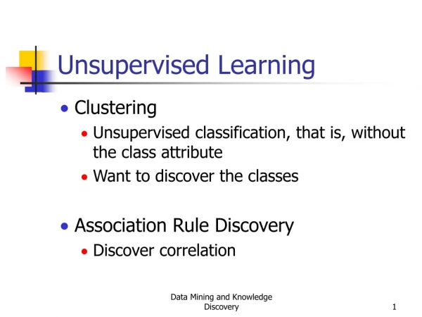
Clustering Methods without Labels • Try to discover the hidden information about the unlabeled data • Also to discover the relationship among data • The common analytical method is the clustering method • One classical unsupervised learning methods • Divide data into meaningful or useful groups • Called clusters • Grouping similar data objects as clusters • All clustering methods are based on similarity testing • Unlike supervised classification, the groups are not known in advance
Clustering Methods without Labels • Making this an unsupervised task • For data analysis, cluster is the potential class • Clustering analysis is the technique to find this class automatically • Clustering algorithms • e.g., K-means clustering and density-based clustering methods • Density estimation finds the distribution of inputs in some space
Cluster Analysis for Prediction and Forecasting • Cluster analysis assigns a set of observations to partition a data set into clusters • Based on a Euclidean distance or similarity function • Aimed to separate data for classification purpose • Data elements grouped into the same cluster • Similar or have some common properties • According to a predefined similarity metric • The clusters are separated by dissimilar features or properties • Other clustering methods are based on estimated density and graph connectivity
Cluster Analysis for Prediction and Forecasting (cont.) • Cluster analysis is a process to divide data objects into clusters • X is the set of n data objects • Xi the cluster label • The clusters are the disjoint subsets • Cluster Analysis of Hospital Exam Records • The physical examination groups are divided into conformity group and nonconformity group • Based on clustering of characteristics • Nonconformity may be divided into subgroups • With hyperlipidemia or with heart disease
Cluster Analysis for Prediction and Forecasting (cont.) • The group with hyperlipidemia is divided into • High-risk and low-risk subgroups
Cluster Analysis for Prediction and Forecasting (cont.) • The difference between clustering and classification • Clustering-based division is uncertain • From the perspective of machine learning • Clustering is an unsupervised learning process with a constant search for clusters • Clustering requires determination of the labels by user • The classification is a supervised learning process to divide existing objects into different groups with various labels • How to do clustering for given certain datasets requires the design of specific algorithms • K-means clustering is a basic clustering method
K-means Clustering for Classification • Groups a large set of unrelated data elements (or vectors) into k clusters • Assume that the dataset D contains n objects in Euclidean space • Need to divide objects in the D into k clusters • C1, C2,⋯, Ck, making 1 ≤ i, j ≤ k, Ci ⊂ D, Ci∩ Cj = ∅ • Necessary to evaluate the quality of the division • Defining an objective function with the object of high similarity in a cluster and low inter-cluster similarity • To embody a cluster more visually • The centroid heart of a cluster represents the cluster
K-means Clustering for Classification (cont.) • ni denotes the number of elements in a cluster • denotes the vector coordinate of cluster elements • denotes the centroid’s coordinates of Ci • Use d(x, y) to denote the Euclidean distance between the two vectors • The objective function • The error sum of squares of all objects in data sets D to the centroid of a cluster • The objective of K-means clustering • For a given dataset and given k • Find a group of clusters C1, C2,⋯, Ck to minimize the objective function E
K-means Clustering for Classification (cont.) • K-means clustering is implemented with an iterative refinement technique • Also known as Lloyd’s Algorithm • Let S be the set of n data elements • Si is the i-th cluster subset • The clusters, Si for i = 1, 2, … k, are disjoint subsets of S forming a partition of the data set S • Given an initial set of k means • The algorithm proceeds by alternating between • Assignment step
K-means Clustering for Classification (cont.) • Assign each observation to the cluster with mean being the centroid of set Si to yield the least within-cluster sum of squares (WCSS) • The squared Euclidean distance at time t = 1, 2,.… • Update step • Calculate the new means at time step t+1 as the centroids of the observations in the new clusters • The arithmetic mean minimizes the WCSS • This algorithm will converge when the assignments no longer reduce the WCSS • Both above steps optimize the WCSS objective
K-means Clustering for Classification (cont.) • Only a finite number of iterations to yield the final partitioning • The algorithm must converge to a (local) optimum • The idea is to assign data objects to the nearest cluster by distance • The K-mean Clustering method
K-means Clustering for Classification (cont.) • Using K-mean Clustering to Classify Patients into Three Clusters • Hyperlipidemia is a common disease • Due to high levels of blood lipids • The contents of triglyceride and total cholesterol in the blood are always used to determine this disease • According to the two above indexes, people can be divided into two categories • i.e. Normal people and patients with the disease • The dataset of triglyceride and total cholesterol contents of physical examinations in a hospital • To divide these people into different groups, it is necessary to conduct cluster analysis
K-means Clustering for Classification (cont.) • All the datasets can be obtained as • First determine the number of clusters • Need to divide into three groups, identified by k = 3
K-means Clustering for Classification (cont.) • Then necessary to select three objects randomly to constitute the initial cluster • Select the objects in D as per the nearest Euclidean distance • Put them into the three clusters above • e.g., For object e = (1.33, 4.19), the Euclidean distances of the object to the three clusters
K-means Clustering for Classification (cont.) • Thus object e is nearest to the cluster C2 • It should be divided into the cluster C2 • In this way to obtain the three clusters • Then recalculate the mean of cluster objects
K-means Clustering for Classification (cont.) • Reallocate each object of the dataset D in the similar way into each cluster • The mean values and relocated means can be very close to terminate the process • Ends up with the final classification • These physically examined people in this hospital can be grouped into three categories • i.e., Normal people, people with slight symptoms or having potential to become sick, and people with hyperlipidemia
K-means Clustering for Classification (cont.) • Construct the clusters iteratively • The initial choice of centroids and four steps to build three clusters out of 15 data points • k initial means are randomly generated within the data domain • In this case k = 3 • k clusters are created by associating each data point with the nearest mean • The partitions correspond to the Voronoi diagram generated by the means • The centroid of each of the k clusters becomes the new mean • Steps 2 and 3 are repeated until convergence has been reached
K-means Clustering for Classification (cont.) • Using K-Means Clustering to Classify Iris • Solving an iris flower classification problem • With k-means clustering for k = 3 clusters • Given a data set of 150 unlabeled data points on iris flowers • These flowers are classified into three clusters • Iris setosa, Iris versicolour, and Iris virginica
K-means Clustering for Classification (cont.) • There are four features in this data set • Sepal length in cm, sepal width in cm, petal length in cm, and petal width in cm • Only consider the data points with the last two most important features • Identify the clustering centers (centroids) in successive steps • Get the final means after two iterations
K-means Clustering for Classification (cont.) • The k-means clustering in R code