Cascade Correlation
Learn about the cascade correlation algorithm in neural networks, specifically focusing on radial basis functions. Explore weight training, covariance optimization, and clustering in input space. Understand linear interpolation for function approximation in one and multiple dimensions.

Cascade Correlation
E N D
Presentation Transcript
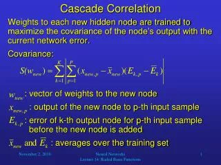
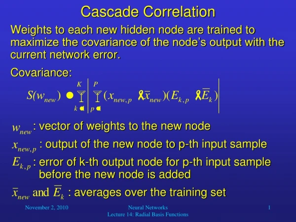
Cascade Correlation • Weights to each new hidden node are trained to maximize the covariance of the node’s output with the current network error. • Covariance: : vector of weights to the new node : output of the new node to p-th input sample : error of k-th output node for p-th input sample before the new node is added : averages over the training set Neural Networks Lecture 14: Radial Basis Functions
Cascade Correlation • Since we want to maximize S (as opposed to minimizing some error), we use gradient ascent: : i-th input for the p-th pattern : sign of the correlation between the node’s output and the k-th network output : learning rate : derivative of the node’s activation function with respect to its net input, evaluated at p-th pattern Neural Networks Lecture 14: Radial Basis Functions
Cascade Correlation • If we can find weights so that the new node’s output perfectly covaries with the error in each output node, we can set the new output node weights and offsets so that the new error is zero. • More realistically, there will be no perfect covariance, which means that we will set each output node weight so that the error is minimized. • To do this, we can use gradient descent or linear regression for each individual output node weight. • The next added hidden node will further reduce the remaining network error, and so on, until we reach a desired error threshold. Neural Networks Lecture 14: Radial Basis Functions
Cascade Correlation • This learning algorithm is much faster than backpropagation learning, because only one neuron is trained at a time. • On the other hand, its inability to retrain neurons may prevent the cascade correlation network from finding optimal weight patterns for encoding the given function. Neural Networks Lecture 14: Radial Basis Functions
Input Space Clusters • One of our basic assumptions about functions to be learned by ANNs is that inputs belonging to the same class (or requiring similar outputs) are located close to each other in the input space. • Often, input vectors from the same class form clusters, i.e., local groups of data points. • For such data distributions, the linearly dividing functions used by perceptrons, Adalines, or BPNs are not optimal. Neural Networks Lecture 14: Radial Basis Functions
Input Space Clusters Circle 1 Line 3 • Example: x2 Line 4 Class 1 Class -1 x1 Line 1 Line 2 A network with linearly separating functions would require four neurons plus one higher-level neuron. On the other hand, a single neuron with a local, circular “receptive field” would suffice. Neural Networks Lecture 14: Radial Basis Functions
Radial Basis Functions (RBFs) • To achieve such local “receptive fields,” we can use radial basis functions, i.e., functions whose output only depends on the Euclidean distance between the input vector and another (“weight”) vector. • A typical choice is a Gaussian function: • where c determines the “width” of the Gaussian. • However, any radially symmetric, non-increasing function could be used. Neural Networks Lecture 14: Radial Basis Functions
Linear Interpolation: 1-Dimensional Case • For function approximation, the desired output for new (untrained) inputs could be estimated by linear interpolation. • As a simple example, how do we determine the desired output of a one-dimensional function at a new input x0 that is located between known data points x1 and x2? • which simplifies to: • with distances D1 and D2 from x0 to x1 and x2, resp. Neural Networks Lecture 14: Radial Basis Functions
Linear Interpolation: Multiple Dimensions • In the multi-dimensional case, hyperplane segments connect neighboring points so that the desired output for a new input x0 is determined by the P0 known samples that surround it: • Where Dp is the Euclidean distance between x0 and xp and f(xp) is the desired output value for input xp. Neural Networks Lecture 14: Radial Basis Functions
Linear Interpolation: Multiple Dimensions • Example for f:R2R1 (with desired output indicated): • For four nearest neighbors, the desired output for x0 is D3 D2 D6 D7 X0 : ? X3 : 4 X1 : 9 X2 : 5 X4 : -6 X7 : 6 X8 : -9 X6 : 7 X5 : 8 Neural Networks Lecture 14: Radial Basis Functions