Download

1 / 123
1.26k likes | 1.5k Vues
ON ESTIMATING THE URBAN POPULATIONS USING MINIMUM INFORMATION. Arun Kumar Sinha Department of Statistics Central University of Bihar Patna 800 014, Bihar INDIA ( arunkrsinha@yahoo.com ) 08 October, 2014 IAOS 2014 Conference Da Nang, Vietnam. Abstract

E N D
ONESTIMATING THE URBAN POPULATIONS USING MINIMUM INFORMATION Arun Kumar Sinha Department of Statistics Central University of Bihar Patna 800 014, Bihar INDIA (arunkrsinha@yahoo.com) 08 October, 2014 IAOS 2014 Conference Da Nang, Vietnam
Abstract • For implementing the programmes and policies of the urban planning department we need to know the current populations of the urban areas of interest. • Many times the required information is not easily available.
In view of these scenarios the paper deals with some techniques of estimating the populations of urban areas when only the minimum information is available. • The real data sets are used to illustrate the methods that provide some interesting and useful results. • This paper could be of immense help to the planners and decision makers of the urban areas related issues.
MAIN STEPS IN A SAMPLING • Identification • Acquisition • Quantification
FAMILIAR DILEMMA IN SAMPLING • We need large sample sizes for adequately representing heterogeneous populations. [Desirability] • But our budget permits only a limited number of measurements. [Affordability] • We refer to this “best of both worlds” scenarios as observational economy.
OBSERVATIONAL ECONOMY • For observational economy to be feasible, identification and acquisition of sampling units should be inexpensive as compared with their quantification. • Ranked set sampling (RSS) is one such method for achieving observational economy.
RANKED SET SAMPLING • McIntyre (1952) proposed a method of sampling for estimating pasture yields. He referred to it as “a method of unbiased selective sampling using ranked sets”. • The present name, “ranked set sampling” (RSS), was coined by Halls and Dell (1966).
Ranked set sampling is useful in situations in which measurements are difficult or costly to obtain but ranking of a subset of units is relatively easy. • It aims to achieve what stratified sampling cannot in real-life situations, i.e. adequately representing a population.
BASIC IDEAS • A fairly large random collection of sampling units is portioned into small subsets, each subset being of size m, say. • Each subset is ranked as accurately as possible with respect to the characteristic of interest without using its exact measurement, and exactly one member of each set with certain specification is quantified.
Thus, only a fraction 1/m of the collection of sampling units is quantified for achieving observational economy.
SOME USEFUL RANKING CRITERIA • Visual perception / Inspection (Colour, Odour, Distressed Vegetation, Distressed Ground, Oily Sheens, Manmade Structures, Surface Water and Groundwater Flow Direction, Wind Direction, etc.) • Prior Information • Results of earlier sampling episodes • Rank-correlated covariates • Expert-opinion/expert-systems • Some combination of these methods, etc.
ILLUSTRATION • Suppose we need to draw a sample of three trees from the nine randomly identified trees as shown on the next slide.
We need to rank the three trees of each group (set) visually with respect their heights and take the measurements of the smallest tree from the first group, of the second smallest from the second group and of the tallest tree from the last group. • This yields three measurements representing three independent order statistics. • The three trees whose heights are to be measured are shown on the next slide.
For a larger sample size (n) we repeat the process. With the set size as “m” and the number of cycles as “r”, we obtain the sample size, n = mr. For getting a sample of size 6 with set size 3, we need to have 2 cycles. LARGER SAMPLE SIZE
STEPS FOR DRAWING A RANKED SET SAMPLE • Randomly select m2 units from the population. • Allocate the m2 selected units as randomly as possible into m sets each of size m. • Rank the units within each set based on a perception of relative values of the variable of interest.
Choose a sample by including the smallest ranked unit of the first set, then the second smallest ranked unit of the second set, continuing in this fashion until the largest ranked unit is selected from the last set. • Repeat steps (1) through (4) for r cycles until the desired sample size, n = mr, is obtained for analysis.
Let X11, X12, …, X1m; X21, X22, … , X2m; … , Xm1, Xm2, … , Xmm be independent random variables having the same cumulative distribution function F(x). • The Xij for the randomly drown units can be arranged as in the following diagram:
Set • 1 X11 X12 … X1m • 2 X21 X22 … X2m • . • . • . • m Xm1 Xm2 … Xmm • After ranking the units appear as • 1 X1(1) X1(2) … X1(m) • 2 X2(1) X2(2) … X 2(m) • . • . • . • m Xm(1) Xm(2) … Xm(m)
The units to be quantified are presented below: • 1 X1(1) * … * • 2 * X2(2) … * • . • . • . • m * * … Xm(m)
FIRST, SECOND AND THIRD ORDER OF NORMAL AND EXPONENTIAL DISTRIBUTIONS SOURCE:PATIL, SINHA AND TAILLIE (1994A)
FIRST, SECOND AND THIRD ORDER OF LOGNORMAL AND UNIFORM DISTRIBUTIONS SOURCE:PATIL, SINHA AND TAILLIE (1994A)
Let denote the ith order statistic in the jth cycle, where i = 1, 2, . . . , m and j = 1, 2, . . . , r . Here the sample size n = mr. Further, we observe that
This reveals that all mr quantifications are independent but they are identically and independently distributed (iid) within each row only. The RSS estimator of the population mean is given by
RELATIVE PRECISION • The relative precision (RP) of the ranked set sample (RSS) estimator of the population mean relative to the corresponding simple random sample (SRS) estimator with the same sample size (mr) is given by
where 1 ≤ RP ≤ (m+1)/2
Relative Savings: As RS >= 0 => RSS is at least as cost efficient as SRS with the same number of quantifications.
IMPLEMENTATION OF RSS • The implementation of RSS needs only the rankings of the randomly selected units, and in no way depends upon the method employed for determining the rankings. Thus, investigators can use any or all available information including subjective judgment for this purpose.
Note that other sampling methods such as ratio and regression methods require very detailed model specifications for the outside information. These methods can be highly non-robust to violations of those specifications.
One of the strengths of RSS is its flexibility and model robustness regarding the nature of the auxiliary information used to perform the ranking. • For RSS to be cost effective, the quantification of sampling units rather than their identification, acquisition, and ranking should be the dominant factor of the total cost.
RSS WITH CONCOMITANT RANKING • RSS presumes that the sampling units are correctly ranked with respect to the variable of interest. • But this may not be possible always while dealing with real life situations. In these cases one could take help of some other characteristic for ranking, which is supposedly inexpensive, easily available and highly correlated with the main characteristic of interest.
RSS WITH CONCOMITANT RANKING • The ranking so obtained may be referred to as concomitant ranking (CR) because of its dependence on a concomitant variable. • In classical sampling this is called as an auxiliary variable, and we may denote it by Y while the main variable is represented by X. See Patil, Sinha and Taillie (1994a and b) and Sinha (2005) for a more detailed discussion.
RSS WITH CONCOMITANT RANKING • In order to obtain the expressions of the variances of the three RSS estimators under concomitant ranking we assume that there is a linear relationship between the main variable X and the concomitant variable Y. This yields that
RSS METHODS WITH CONCOMITANT RANKING • where X [i: m] denotes the ith order statistic of X based on a concomitant ranking whereas Y (i: m) shows the ith order statistic of Y based on perfect ranking. • Thus, the expression
RSS METHODS WITH CONCOMITANT RANKING • This leads to the following expression for the var (X [i: m]) for the standard bivariate normal distribution:
The Takahasi’s method is slightly less efficient than the McIntyre’s method. But the former has a number of advantages that make it more suitable to the requirements of sampling and monitoring situations.
RSS WITH SKEWED POPULATIONS • For skewed populations, RSS with the unequal allocation following Neyman’s criterion gives better performance than that with equal allocation. (See Takahasi and Wakimoto (1968). • Accordingly, if ri denotes the number of quantifications of units having rank i then
Then, where r1 + r2 + … + rm = n.
Set m Units 1 ● ○ … r1 2 ● ○ … . . . r1 ● ○ … ● ○ …
Set m Units 1 ○ ● … r2 2 ○ ● … . . . r2 ○ ● …
Set m Units 1 ... ● rm 2 ... ● . . . rm ... ● ... ● . . .