
Group Analysis
E N D
Presentation Transcript
Group Analysis ‘Ōiwi Parker Jones SPM Course, London May 2015
Overview • Variation may come from multiple sources • Some common to all data, e.g. measurement noise • Some common to subsets, e.g. subject variability • How do we model this?
Subject 1 For voxel v in the brain Effect size, c ~ 4
Subject2 For voxel v in the brain Effect size, c ~ 2
Subject 12 For voxel v in the brain Effect size, c ~ 4
Random effect analysis (RFX) >> c = [4, 2, 3, 1, 1, 2, 3, 3, 3, 2, 4, 4]; >> m = mean(c) % mean effect size >> s_b = std(c) % between subject variability >> n = length(c) % number of samples >> sem = s_b / sqrt(n) % standard error of the mean >> t = m / sem % t-stat >> [~,p] = ttest(c,0) % p-value
Random effect analysis (RFX) >> c = [4, 2, 3, 1, 1, 2, 3, 3, 3, 2, 4, 4]; >> m = mean(c) % 2.67 >> s_b = std(c)% 1.07 >> n = length(c) % 12 >> sem = s_b / sqrt(n) % 0.31 >> t = m / sem% 8.61 >> [~,p] = ttest(c,0) % 10-6
Subject 1 For voxel v in the brain Effect size, c ~ 4Within subject variability, sw~0.9
Subject2 For voxel v in the brain Effect size, c ~ 2Within subject variability, sw~1.5
Subject 12 For voxel v in the brain Effectsize, c ~ 4Withinsubjectvariability, sw~1.1
Fixed effects analysis (FFX) >> s_w = [0.9, 1.5, 1.2, 0.5, 0.4, 0.7, 0.8, 2.1, 1.8, 0.8, 0.7, 1.1] >> m = mean(c) % mean effect size >> s_w = mean(s_w)% mean s_w >> n = length(c)*50 % number of samples >> sem= s_w/ sqrt(n) % standard error of the mean >> t = m / sem% t-stat >> [~,p] = ttest(c,0) % p-value
Fixed effects analysis (FFX) >> s_w = [0.9, 1.5, 1.2, 0.5, 0.4, 0.7, 0.8, 2.1, 1.8, 0.8, 0.7, 1.1] >> m = mean(c) % 2.67 >> s_w = mean(s_w) % 1.04 >> n = length(c) * 50% 600 = 12 subj x 50 scans >> sem= s_w/ sqrt(n) % 0.04 >> t = m / sem% 62.7 >> [~,p] = ttest(c,0) % 10-51 “The fallacy of classical inference”
n= 600 sw …
n= 12 Subj 1 Subj 2 Subj 12 sb …
Summary stats First level DataDesign MatrixContrast Images
Summary stats First level Second level DataDesign MatrixContrast Images SPM(t) One-sample t-test @ 2nd level
Hierarchical model (1) Withinsubjectvariance, sw(i)(2) Betweensubjectvariance,sb = + + = Second level First level
Summary stats vshierarchical models • Most people use summary stats (for RFX in neuroimaging) • Quick to compute • Equivalent to hierarchical models if • within-subject variances are the same • 1st level designs are the same (e.g. equal number of trials) • Hierarchical models • Guarantee optimal analysis for each dataset • Can be very useful if • assumptions 1, 2 above are violated (e.g. patient studies) • you want to check your results
Auditory example Summary statistics Hierarchical Model Friston et al. (2004) Mixed effects and fMRI studies, Neuroimage
Multiple conditions (part 1) Condition 1 Condition 2 Condition 3Sub1 Sub13 Sub25Sub2 Sub14 Sub26... ... ...Sub12 Sub24 Sub36ANOVAat 2nd level(e.g. drug).
Multiple conditions (part 2) Condition 1 Condition 2 Condition3Sub1 Sub1 Sub1Sub2 Sub2 Sub2... ... ...Sub12 Sub12 Sub12‘ANOVA withinsubjects’at2nd level.(This is an ANOVA but withaveragesubjecteffectsremoved.)
Summary • Group analysis can be used to model different sources of variation in data, either common (FFX) or not (RFX) • Group inference usually proceeds with RFX, not FFX. Group effects are compared between, rather than within, subject variability. • Hierarchical models provide a gold standard for RFX analysis but are computationally intensive (spm_mfx). • Summary statistics are a robust method for RFX group analysis (see SPM book; Mumford and Nichols, NI, 2009). • This approach is flexible: use ‘ANOVA’ or ‘ANOVA within subject’ at 2nd level for inferences about multiple experimental conditions.