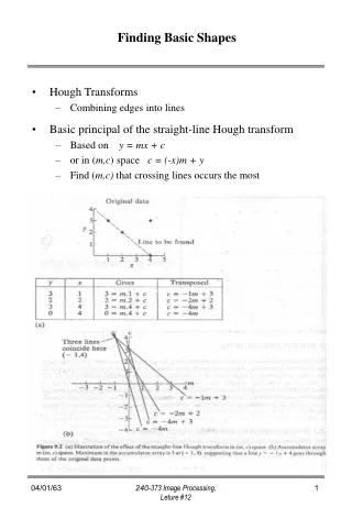
1. Finding Basic Shapes • Hough Transforms • Combining edges into lines • Basic principal of the straight-line Hough transform • Based on y = mx + c • or in (m,c) space c = (-x)m + y • Find (m,c) that crossing lines occurs the most 240-373 Image Processing, Leture #12

2. Real straight-edge discovery using the Hough transform • Problem with the basic technique: m could be from -infinity to +infinity • Polar coordinates can be used instead of cartesian coordinates 240-373 Image Processing, Leture #12

3. Real straight-edge discovery Technique 1: Real straight-edge discovery using the Hough transform USE: To find out and connect substantial straight edges from partial edges already found using an edge detector. OPERATION: • For each edge pixel value I(x,y) , vary q from 0o to 360o and calculate r = x cos q + y sin q • Given an accumulator array size (N + M, 360), increase those elements in the array that lie in a box (b x b) with center (r, q) • Look for the highest values in the accumulator (r, q) array and identify the pairs (r, q) that are the most likely to indicate a line in (x,y) space This method can be enhanced in a number of ways: 1. The gradient of the edge before thresholding can be used to update the accumulator array. 2. Gradient direction can be taken in to account. If this suggests that the direction of the real edge lies between two angles (q1, q2), then only the element in the (r, q) array that lies in q1 < q <q2 are plotted 3. The incrementing box does not need to be uniform. The center can be emphasized 240-373 Image Processing, Leture #12

4. Real Circle Discovery Technique 2: Real circle discovery using the Hough transform USE: To find circles from an edge-detected image. OPERATION: • To search for circles of a known radius, R, then the following identity can be used (x-a)2 + (y-b)2 = R2 where (a,b) is the center of the circle • A circle of elements is incremented in the (a,b) accumulator array center (a = 0 .. M-1, b = 0 .. N-1) • The highest values in the (a,b) array indicates coincident edges 240-373 Image Processing, Leture #12

5. Real circle discovery (cont’d) • It is possible to look for the following types of circle: • different radii plot in (a,b,R) space • different radii, same vert. centers plot in (b,R) space • different radii, same horz. centers plot in (a,R) space • Important points • As the number of unknown parameters increases, the amount of processing increases exponentially • The Hough technique can be used to discover any edge shapes with simple identity • The generalized Hough transform can be used to discover complex shapes Technique 2: The generalized Hough transform USE: To find a known shape of any size or orientation in an image. OPERATION: • Given the object boundary (assuming that the object is of the same size and orientation), choose a center (x,y) • The boundary is traversed and after every step d along the boundary the angle of the boundary tangent with respect to horizontal is noted, and the x difference and y difference of the boundary position from the center point are also noted. • See table 240-373 Image Processing, Leture #12

6. For every pixels I(x,y) in the edge-detected image, the gradient direction is found • and the row of elements in the array shown in the table above then refer to a set of elements relative to this boundary point which may be ‘center’ of the object • The accumulator (same size as image) is then incremented by 1 for such element • Finally, the highest-valued element(s) in the accumulator array point to the possible ‘centers’ of the object 240-373 Image Processing, Leture #12

7. Bresenham’s algorithms • Bresenham’s straight-line drawing algorithm • Bresenham’s circle drawing algorithm 240-373 Image Processing, Leture #12

8. 240-373 Image Processing, Leture #12

9. 240-373 Image Processing, Leture #12