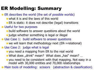
ER Modelling: Summary

1. ER Modelling: Summary • ER describes the world (the set of possible worlds) • what it is and the laws of this world • ER is static: it does not describe (legal) transitions • Useful for two purposes • build software to answer questions about the world • judge whether something is legal or illegal • Use Case 1: build software to answer questions • we will learn that methodology next (ER->relational) • Use Case 2: judge what is legal • you need a mapping from ER to the real world • What does „drink“ mean? What does „has“ mean? … • you need to be consistent with that mapping. Not easy in a model with 30,000 entities and 70,000 relationships • Main tools of modelling: scissors (abstraction & classification)

2. Relational Data Model Relation: R  D1 x ... x Dn D1, D2, ..., Dn are domains Example: AddressBook  string x string x integer Tuple: t  R Example: t = („Mickey Mouse“, „Main Street“, 4711) Schema: associates labels to domains Example: AddrBook: {[Name: string, Address: string, Tel#:integer]}

3. Instance:the state of the database • Key:minimal set of attributes that identify each tuple uniquely • E.g., {Tel#} or {Name, BirthDate} • Primary Key:(marked in schema by underlining) • select one key • use primary key for references

4. requires Uni-Schema follow- up Nr Legi prerequisite N M attends CP Lecture Name Student N M N N Title Semester M gives tests Grade PersNr 1 1 Level Works-for Name Assistant Professor Room N 1 Area PersNr Name

5. Rule #1: Implementation of Entities Student: {[Legi:integer, Name: string, Semester: integer]} Lecture: {[Nr:integer, Title: string, CP: integer]} Professor: {[PersNr:integer, Name: string, Level: string, Room: integer]} Assistant: {[PersNr:integer, Name: string, Area: string]}

6. Rule #2: Relationships A11 E1 ... AR1 R ... A21 E2 En ... An1 ... ... R:{[ ]}

7. Implementation of Relationships attends : {[Legi: integer, Nr: integer]} gives : {[PersNr: integer, Nr: integer]} works-for : {[AssistentPersNr: integer, ProfPersNr: integer]} requires: {[prerequisite: integer, follow-up: integer]} tests : {[Legi: integer, Nr: integer, PersNr: integer, Grade: decimal]}

8. Instance of attends Nr Legi N M Student Lecture attends

9. Rule 2: How to call the attributes • If the ER specifies roles • use the names of the roles • Otherwise • use the names of the key attributes in the entities • in case of ambiguity, invent new names • Example: friend : {[ProfNr: integer, AssiNr: integer]} friend Assistant Professor M N PersNr PersNr

10. Exercise • Implement the following ER diagram using the rel. data model Number 1 1 1 plus

11. Rule #3: Merge relations with the same key gives Lecture Professor N 1 • Implementation according to Rule #2 Lecture :{[Nr, Title, CP]} Professor :{[PersNr, Name, Level, Room]} gives:{[Nr, PersNr]} • Merge according to Rule #3 Lecture :{[Nr, Title, CP, PersNr]} Professor :{[PersNr, Name, Level, Room]} Why is this better? When can this be done? • „Zusammenwachsen, was zusammen gehört!“ 1

12. Instance of Professor and Lecture gives Lecture Professor N 1

13. This will NOT work gives Lecture Professor N 1

14. This will NOT work Problem: Redundancy and Anomalies PersNr is no longer key of Professor (issue will be revisited when we talk about normal forms)

15. Rule #4: Generalization Area Assistant is_a Employee Professor PersNr Name Room Level

16. Rule #4: Generalization Area Assistant is_a Employee Professor PersNr Name Room Level Employee: {[PersNr, Name]} Professor: {[PersNr, Level, Room]} Assistant: {[PersNr, Area]}

17. Rule #4: Generalization-alternative Area Assistant is_a Employee Professor PersNr Name Room Level Employee: {[PersNr, Name]} Professor: {[PersNr, Name, Level, Room]} Assistant: {[PersNr, Name, Area]} What is better?

18. Rule #5: Weak Entities Grade N Student 1 takes Exam Part N N Legi covers gives PersNr Nr M M Lecture Professor Exam: {[Legi: integer, Part: string, Grade: integer]} covers: {[Legi: integer, Part: string, Nr: integer]} gives: {[Legi: integer, Part: string, PersNr: integer]}

19. Weak Entities in detail: „takes“ • takes: {[StudiLegi: int, ExamLegi: int, Part: string, Nr: int]} • What is/are the key(s) of the „takes“ relation? • Why can it be merged with the „Exam“ relation (Rule #3)? • What happened to the „StudiLegi“ column as part of this merge?

20. Food for Thought: OO vs. Relations • How do Java and C++ implement ER? • Are they a better match than the relational model? • Specifically, how do Java and C++ implement Generalization? • Is it good or bad to have several possible ways? • Concept of Reference: Compare Java and Relational Model • Which one is better? • Life-time of objects: Compare Java and Relational Model • Why different?

21. Relational Model of Uni-DB

22. Relational Algebra  Selection  Projection X Cartesian Product A Join  Rename  Set Minus  Relational Division  Union  Intersection F Semi-Join (left) E Semi-Join (right) C left outer Join D right outer Join

23. Formal Definition of Rel. Algebra Atoms (basic expressions) • A relation in the database • A constant relation Operators (composite expressions) • Selection: p (E1) • Projection: S (E1) • Cartesian Product: E1 x E2 • Rename: V (E1), A  B (E1) • Union: E1 E2 • Minus: E1- E2

24. Selection and Projection Semester > 10 (Student) Selection Level(Professor) Projection

25. Cartesian Product = x

26. Cartesian Product (ctd.) Professor x attends • Huge result set (n * m) • Usually only useful in combination with a selection (-> Join)

27. Natural Join Two relations: • R(A1,..., Am, B1,..., Bk) • S(B1,..., Bk, C1,..., Cn) R A S = A1,..., Am, R.B1,..., R.Bk, C1,..., Cn(R.B1=S. B1 ... R.Bk = S.Bk(RxS))

28. Three-way natural Join (Student A attends) A Lecture

29. Theta-Join Two Relations: • R(A1, ..., An) • S(B1, ..., Bm) R A  S =  (R x S) R AS

30. Theta Join Example • Train(name, start, destination, …, length) • Track(station, number, …, length) • Find all possible tracks for the „CIS Alpino“ in Zurich station=„Zurich“(Track) A Train.length < Track.lengthname=„CIS“(Train) Source: anonymous student from the 2011 class

31. Join Variants • natural join A = • left outer join C =

32. Join Variants • right outer join D =

33. Join Variants • (full) outer join B = • left semi join E =

34. Join Variants • right semi join F =

35. Rename Operator Rename operator: r • Renaming of relation names • Needed to process self-joins and recursive relationships • E.g., two-level dependencies of lectures („grandparents“) L1.Prerequisite(L2. Follow-up=5216  L1.Follow-up = L2.Prerequisite (L1 (requires) x L2 (requires))) • Renaming of attribute names Requirement  Prerequisite (requires)

36. Intersection • Only works if both relations have the same schema • Same attribute names and attribute domains • Intersection can be simulated with minus: R  S = R  (R  S) PersNr(Lecture)  PersNr(Level=FP(Professor))

37. Relational Division Find students who attended all lectures with 4CP. attends  Nr(CP=4(Lecture))

38. Definition of Division • t  R  S, iff for each ts  S exists a tr  R such that: • tr.S = ts.S • tr.(R-S) = t • Division can be simulated with other operators:  = R  S = (R  S)(R)   (R  S)(( (R  S)(R) x S)  R)

39. Division: Example • R = attends; S = Lecture • Legi(attends)All students (who attend at least one lecture) • Legi(attends)x LectureAll students attend all lectures • (Legi(attends)x Lecture) – attendsLectures a student does not attend • Legi((Legi(attends)x Lecture) – attends):Students who miss at least one lecture • Legi(hören) - Legi((Legi(attends)x Lecture) – attends)Students who attend all lectures • What happens if there are no lectures or no attendance? R  S = (R  S)(R)   (R  S)(( (R  S)(R)x S)  R)

40. Relational Calculus Queries have the following form: {t  P(t)} with t a variable, P(t) a predicate. Examples: • All full professors {p  p  Professor  p.Level = ‚FP'} • Students who attend at least one lecture of Curie {s s  Student  a  attends(s.Legi=a.Legi  l  Lecture(a.Nr=l.Nr  p  Professor(p.PersNr=l.PersNr  p.Name = 'Curie')))}

41. Who attends all lectures with 4 CP? {s  s  Student  l  Lecture (l.CP=4  a  attends(a.Nr=l.Nr  a.Legi= s.Legi))} There are two variants of relational calculus: tuple relational calculus (as in examples above, tuple vars) domain relational calculus (variables iterate over domains)

42. Definition des Tuple Relational Calculus Atoms • s  R • s is a tuple variable, R is a name of a relation • s.A t.B or s. A  c • s and t tuple variables, A and B attribute names  a comparison (i.e., , , , ...) • c is a constant (i.e., 25) Formulas • All atoms are legal formulas • If P is a formula, then P and (P) are also formulas • If P1 and P2 are formulas, then P1  P2 , P1  P2 and P1  P2 • If P(t) is a formula with a free variable t, then t  R(P(t)) and  t  R(P(t))

43. Safety • Restrict formulas to queries with finite answers • Semantic not syntactic property! • Example: The following expression is not safe {n   (n  Professor)} • Definition of safety • result must be subset of the „domain of the formula“ • „domain of the formula“ • All constants used in the formula • All domains of relations used in the formula

44. Domain Relational Calculus An expression has the following form {[v1, v2 , ..., vn]P (v1 ,..., vn)} each v1 ,..., vn is either a domain variable or a constant. P is a formula. Example: Legi and Name of all students tested by Curie: {[l, n]  s ([l, n, s]  Student  v, p, g ([l, v, p, g]  tests  a,r, b([p, a, r, b]  Professor  a = 'Curie')))}

45. Safety in the DRC • Defined in same way as for tuple relational calculus • Example: The following expression is not safe {[p,n,r,o]   ([p,n,r,o]  Professoren) } • (see text book for exact definition of safety in DRC)

46. Codd`s Theorem The three languages • relational algebra, • tuple relational calculus (safe expressions only) • domain relational calculus (safe expressions only) are equivalent Impact of Codd`s theorem • SQL is based on the relational calculus • SQL implementation is based on relational algebra • Codd`s theorem shows that SQL implementation is correct and complete.