Relational Calculus and Datalog

1. Relational Calculus and Datalog Helena Galhardas DEI IST (Slides baseados No Cap 5 livro DB Concepts Silberchatz et al, e disciplina CSE330 – Database Management Systems, Susan B. Davidson)

2. Agenda • Tuple Relational Calculus • Domain Relational Calculus • Datalog

3. Codd’s Relational Algebra • A set of mathematical operators that compose, modify, and combine tuples within different relations • Relational algebra operations operate on relations and produce relations (“closure”) f: Relation  Relation f: Relation x Relation  Relation

4. A Set of Logical Operations: The Relational Algebra • Six basic operations: • Projection  (R) • Selection  (R) • Union R1[ R2 • Difference R1 – R2 • Product R1£ R2 • (Rename) ->b (R) • And some other useful ones: • Join R1⋈ R2 • Semijoin R1 sj R2 • Intersection R1Å R2 • Division R1¥ R2

5. Switching Gears: An Equivalent, ButVery Different, Formalism • Codd invented a relational calculus that he proved was equivalent in expressiveness • Based on a subset of first-order logic – declarative, without an implicit order of evaluation • Tuple relational calculus • Domain relational calculus • More convenient for describing certain things, and for certain kinds of manipulations • The database uses the relational algebra internally • But query languages (e.g., SQL) are mostly based on the relational calculus

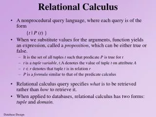
6. Tuple Relational Calculus • A nonprocedural query language, where each query is of the form {t | P (t ) } • It is the set of all tuples t such that predicate P is true for t • t is a tuple variable, t [A ] denotes the value of tuple t on attribute A • t r denotes that tuple t is in relation r • P is a formulasimilar to that of the predicate calculus

7. Predicate Calculus Formula 1. Set of attributes and constants 2. Set of comparison operators: (e.g., , , , , , ) 3. Set of connectives: and (), or (v)‚ not () 4. Implication (): x  y, if x if true, then y is true x  y x v y 5. Set of quantifiers: • t r (Q (t ))”there exists” a tuple in t in relation r such that predicate Q (t ) is true • t r (Q (t )) Q is true “for all” tuples t in relation r

8. Free and Bound Variables • A variable v is bound in a predicate p when p is of the form v… or v… • A variable occurs free in p if it occurs in a position where it is not bound by an enclosing  or  • Examples: • x is free in x > 2 • xis bound inx. x > y

9. Banking Example branch (branch_name, branch_city, assets ) customer (customer_name, customer_street, customer_city ) account (account_number, branch_name, balance ) loan (loan_number, branch_name, amount ) depositor (customer_name, account_number ) borrower(customer_name, loan_number )

10. Example Queries (1) • Find the loan_number, branch_name, and amount for loans of over $1200 {t | t loan  t [amount ]  1200} • Find the loan number for each loan of an amount greater than $1200 {t | s loan (t [loan_number ] = s[loan_number ]  s [amount ]  1200)} Notice that a relation on schema [loan_number ] is implicitly defined by the query

11. Example Queries (2) • Find the names of all customers having a loan, an account, or both at the bank {t |s  borrower ( t [customer_name ] = s [customer_name ])  u  depositor ( t [customer_name ] = u [customer_name ]) • Find the names of all customers who have a loan and an account at the bank {t |s  borrower ( t [customer_name ] = s [customer_name ])  u  depositor ( t [customer_name ] = u [customer_name] )

12. Example Queries (3) • Find the names of all customers having a loan at the Perryridge branch {t |s  borrower (t [customer_name ] = s [customer_name ]  u  loan (u [branch_name ] = “Perryridge”  u [loan_number ] = s [loan_number ]))} • Find the names of all customers who have a loan at the Perryridge branch, but no account at any branch of the bank {t |s  borrower (t [customer_name ] = s [customer_name ]  u  loan (u [branch_name ] = “Perryridge”  u [loan_number ] = s [loan_number ]))  not v  depositor (v [customer_name ] = t [customer_name ])}

13. Example Queries (4) • Find the names of all customers having a loan from the Perryridge branch, and the cities in which they live {t |s  loan (s [branch_name ] = “Perryridge”  u  borrower (u [loan_number ] = s [loan_number ]  t [customer_name ] = u [customer_name ])   v  customer (u [customer_name ] = v [customer_name ]  t [customer_city ] = v [customer_city ])))}

14. Example Queries • Find the names of all customers who have an account at all branches located in Brooklyn: {t | r  customer (t [customer_name ] = r [customer_name ])  ( u  branch (u [branch_city ] = “Brooklyn”   s  depositor (t [customer_name ] = s [customer_name ]   w  account ( w[account_number ] = s [account_number ]  ( w [branch_name ] = u [branch_name ]))))}

15. Safety of Expressions • It is possible to write tuple calculus expressions that generate infinite relations. • For example, { t |  t r } results in an infinite relation if the domain of any attribute of relation r is infinite • To guard against the problem, we restrict the set of allowable expressions to safe expressions. • An expression {t | P (t )}in the tuple relational calculus is safe if every component of t appears in one of the relations, tuples, or constants that appear in P

16. Domain Relational Calculus • A nonprocedural query language equivalent in power to the tuple relational calculus • Each query is an expression of the form: {  x1, x2, …, xn  | P (x1, x2, …, xn)} • x1, x2, …, xn represent domain variables • P represents a formula similar to that of the predicate calculus

17. Example Queries (1) • Find the loan_number, branch_name, and amount for loans of over $1200 { l, b, a  |  l, b, a   loan  a > 1200} • Find the names of all customers who have a loan of over $1200 { c  |  l, b, a ( c, l   borrower   l, b, a   loan  a > 1200)} • Find the names of all customers who have a loan from the Perryridge branch and the loan amount: { c, a  |  l ( c, l   borrower  b ( l, b, a   loan  b = “Perryridge”))} { c, a  |  l ( c, l   borrower   l, “ Perryridge”, a   loan)}

18. Example Queries (2) • Find the names of all customers having a loan, an account, or both at the Perryridge branch: { c  |  l (  c, l   borrower  b,a ( l, b, a   loan  b = “Perryridge”))   a ( c, a   depositor  b,n ( a, b, n   account  b = “Perryridge”))} • Find the names of all customers who have an account at all branches located in Brooklyn: { c  |  s,n ( c, s, n   customer)   x,y,z ( x, y, z   branch  y = “Brooklyn”)   a,b ( x, y, z   account   c,a   depositor)}

19. Safety of Expressions The expression: {  x1, x2, …, xn  | P (x1, x2, …, xn )} is safe if all of the following hold: • All values that appear in tuples of the expression are values from dom (P ) (that is, the values appear either in P or in a tuple of a relation mentioned in P ). • For every “there exists” subformula of the form  x (P1(x )), the subformula is true if and only if there is a value of x in dom (P1) such that P1(x ) is true. • For every “for all” subformula of the form x (P1 (x )), the subformula is true if and only if P1(x ) is true for all values x from dom (P1).

20. Datalog • Basic Structure • Syntax of Datalog Rules • Semantics of Nonrecursive Datalog • Safety • Relational Operations in Datalog • Recursion in Datalog • The Power of Recursion

21. Basic Structure • Prolog-like logic-based language that allows recursive queries; based on first-order logic. • A Datalog program consists of a set of rules that define views. • Examples: • define a view relation v1 containing account numbers and balances for accounts at the Perryridge branch with a balance of over $700. v1 (A, B ) :– account (A, “Perryridge”, B ), B > 700. • Retrieve the balance of account number “A-217” in the view relation v1. ? v1 (“A-217”, B ). • To find account number and balance of all accounts in v1 that have a balance greater than 800? v1 (A,B ), B > 800

22. Example Queries • Each rule defines a set of tuples that a view relation must contain. • v1 (A, B ) :– account (A, “ Perryridge”, B ), B > 700 is read as for allA, B if (A, “Perryridge”, B )  accountand B > 700 then (A, B )  v1 • The set of tuples in a view relation is then defined as the union of all the sets of tuples defined by the rules for the view relation. • Example: interest_rate (A,5):– account (A, N, B ) , B < 10000interest_rate (A,6):– account (A, N, B ), B >= 10000

23. Negation in Datalog • Define a view relation c that contains the names of all customers who have a deposit but no loan at the bank: c(N):– depositor (N, A), not is_borrower (N). is_borrower (N):–borrower (N,L). • NOTE:using notborrower (N, L) in the first rule results in a different meaning, namely there is some loan L for which N is not a borrower. • To prevent such confusion, we require all variables in negated “predicate” to also be present in non-negated predicates

24. Named Attribute Notation • Datalog rules use a positional notation that is convenient for relations with a small number of attributes • It is easy to extend Datalog to support named attributes. • E.g., v1 can be defined using named attributes a v1 (account_number A, balance B ) :– account (account_number A, branch_name “ Perryridge”, balance B ), B > 700.

25. Formal Syntax and Semantics of Datalog • We formally define the syntax and semantics (meaning) of Datalog programs, in the following steps • We define the syntax of predicates, and then the syntax of rules • We define the semantics of individual rules • We define the semantics of non-recursive programs, based on a layering of rules • It is possible to write rules that can generate an infinite number of tuples in the view relation. To prevent this, we define what rules are “safe”. Non-recursive programs containing only safe rules can only generate a finite number of answers. • It is possible to write recursive programs whose meaning is unclear. We define what recursive programs are acceptable, and define their meaning.

26. Syntax of Datalog Rules • A positive literal has the form p (t1, t2 ..., tn ) • p is the name of a relation with n attributes • each tiis either a constant or variable • A negative literalhas the form not p (t1, t2 ..., tn ) • Comparison operations are treated as positive predicates • E.g. X > Y is treated as a predicate >(X,Y ) • “>” is conceptually an (infinite) relation that contains all pairs of values such that the first value is greater than the second value • Arithmetic operations are also treated as predicates • E.g. A = B + C is treated as +(B, C, A), where the relation “+” contains all triples such that the third value is the sum of the first two

27. Syntax of Datalog Rules (Cont.) • Rulesare built out of literals and have the form: p (t1, t2, ..., tn ) :– L1, L2, ..., Lm. head body • each Li is a literal • head – the literal p (t1, t2, ..., tn ) • body – the rest of the literals • A factis a rule with an empty body, written in the form: p (v1, v2, ..., vn ). • indicates tuple (v1, v2, ..., vn )is in relation p • A Datalog program is a set of rules

28. Semantics of a Rule • A ground instantiation of a rule (or simply instantiation) is the result of replacing each variable in the rule by some constant. • Eg. Rule defining v1 v1(A,B):– account (A,“Perryridge”, B ), B > 700. • An instantiation above rule: v1 (“A-217”, 750) :–account ( “A-217”, “Perryridge”, 750), 750 > 700. • The body of rule instantiation R’ is satisfiedin a set of facts (database instance) l if 1. For each positive literal qi (vi,1, ..., vi,ni) in the body of R’, l contains the fact qi (vi,1, ..., vi,ni ). 2. For each negative literal notqj (vj,1, ..., vj,nj ) in the body of R’, l does not contain the fact qj (vj,1, ..., vj,nj ).

29. Semantics of a Rule (Cont.) • We define the set of facts that can be inferredfrom a given set of facts l using rule R as: infer(R, l) = { p (t1, ..., tn)| there is a ground instantiation R’ of R where p (t1, ..., tn )is the head of R’, and the body of R’ is satisfied in l } • Given a set of rules  = {R1, R2, ..., Rn}, we define infer(, l) = infer (R1, l ) infer (R2, l ) ...  infer (Rn, l )

30. Layering of Rules • Define the interest on each account in Perryridge interest(A, l) :– perryridge_account (A,B), interest_rate(A,R), l = B * R/100.perryridge_account(A,B) :– account (A, “Perryridge”, B).interest_rate (A,5) :– account (N, A, B), B < 10000.interest_rate (A,6) :– account (N, A, B), B >= 10000. • Layering of the view relations

31. Layering Rules (Cont.) Formally: • A relation is a layer 1 if all relations used in the bodies of rules defining it are stored in the database. • A relation is a layer 2 if all relations used in the bodies of rules defining it are either stored in the database, or are in layer 1. • A relation p is in layer i + 1 if • it is not in layers 1, 2, ..., i • all relations used in the bodies of rules defining a p are either stored in the database, or are in layers 1, 2, ..., i

32. Semantics of a Program Let the layers in a given program be 1, 2, ..., n. Let i denote the set of all rules defining view relations in layer i. • Define I0 = set of facts stored in the database. • Recursively define li+1 = li infer (i+1, li ) • The set of facts in the view relations defined by the program (also called the semantics of the program) is given by the set of facts lncorresponding to the highest layer n. Note: Can instead define semantics using view expansion like in relational algebra, but above definition is better for handling extensions such as recursion.

33. Safety • It is possible to write rules that generate an infinite number of answers. gt(X, Y) :– X > Y not_in_loan (B, L):– not loan (B, L) To avoid this possibility Datalog rules must satisfy the following conditions: • Every variable that appears in the head of the rule also appears in a non-arithmetic positive literal in the body of the rule. • This condition can be weakened in special cases based on the semantics of arithmetic predicates, for example to permit the rulep (A ) :- q (B ), A = B + 1 • Every variable appearing in a negative literal in the body of the rule also appears in some positive literal in the body of the rule.

34. Relational Operations in Datalog • Project out attribute account_name from account. query (A):–account (A, N, B ). • Cartesian product of relations r1 and r2. query (X1, X2, ..., Xn, Y1, Y1, Y2, ..., Ym ):–r1 (X1, X2, ..., Xn ), r2 (Y1, Y2, ..., Ym ). • Union of relations r1 and r2. query (X1, X2, ..., Xn ) :–r1 (X1, X2, ..., Xn ), query (X1, X2, ..., Xn ) :–r2 (X1, X2, ..., Xn ), • Set difference of r1 and r2. query (X1, X2, ..., Xn ) :–r1(X1, X2, ..., Xn ), notr2 (X1, X2, ..., Xn ),

35. Recursion in Datalog • Suppose we are given a relation manager (X, Y )containing pairs of names X, Y such that Y is a manager of X (or equivalently, X is a direct employee of Y). • Each manager may have direct employees, as well as indirect employees • Indirect employees of a manager, say Jones, are employees of people who are direct employees of Jones, or recursively, employees of people who are indirect employees of Jones • Suppose we wish to find all (direct and indirect) employees of manager Jones. We can write a recursive Datalog program. empl_jones (X ) :- manager (X, Jones ). empl_jones (X ) :- manager (X, Y ), empl_jones (Y ).

36. Semantics of Recursion in Datalog • Assumption (for now): program contains no negative literals • The view relations of a recursive program containing a set of rules  are defined to contain exactly the set of facts l computed by the iterative procedure Datalog-Fixpoint procedure Datalog-Fixpointl = set of facts in the databaserepeatOld_l = l l = l  infer (, l ) until l = Old_l • At the end of the procedure, infer (, l )  l • Infer (, l ) = l if we consider the database to be a set of facts that are part of the program • l is called a fixed pointof the program.

37. Example of Datalog-FixPoint Iteration

38. A More General View • Create a view relation empl that contains every tuple (X, Y ) such that X is directly or indirectly managed by Y. empl (X, Y ):– manager (X, Y ). empl (X, Y ):– manager (X, Z ), empl (Z, Y ) • Find the direct and indirect employees of Jones. ? empl (X, “Jones”). • Can define the view empl in another way too: empl (X, Y ):– manager (X, Y ).empl (X, Y ):– empl (X, Z ), manager (Z, Y).

39. The Power of Recursion • Recursive views make it possible to write queries, such as transitive closure queries, that cannot be written without recursion or iteration. • Intuition: Without recursion, a non-recursive non-iterative program can perform only a fixed number of joins of manager with itself • This can give only a fixed number of levels of managers • Given a program we can construct a database with a greater number of levels of managers on which the program will not work

40. Recursion in SQL • Starting with SQL:1999, SQL permits recursive view definition • E.g. query to find all employee-manager pairs with recursiveempl (emp, mgr ) as (selectemp, mgrfrommanagerunionselect manager.emp, empl.mgrfrommanager, emplwheremanager.mgr = empl.emp )select * fromempl

41. Monotonicity • A view V is said to be monotonic if given any two sets of facts I1 and I2 such that l1 I2, then Ev (I1) Ev (I2 ), where Evis the expression used to define V. • A set of rules R is said to be monotonic ifl1 I2 implies infer (R, I1 )  infer (R, I2 ), • Relational algebra views defined using only the operations:  , |X|  and  (as well as operations like natural join defined in terms of these operations) are monotonic. • Relational algebra views defined using set difference (–) may not be monotonic. • Similarly, Datalog programs without negation are monotonic, but Datalog programs with negation may not be monotonic.

42. Non-Monotonicity • Procedure Datalog-Fixpoint is sound provided the rules in the program are monotonic. • Otherwise, it may make some inferences in an iteration that cannot be made in a later iteration. E.g. given the rulesa :- not b. b :- c. c. Then a can be inferred initially, before b is inferred, but not later. • We can extend the procedure to handle negation so long as the program is “stratified”: intuitively, so long as negation is not mixed with recursion

43. Non-Monotonicity (Cont.) • There are useful queries that cannot be expressed by a stratified program • Example: given information about the number of each subpart in each part, in a part-subpart hierarchy, find the total number of subparts of each part. • A program to compute the above query would have to mix aggregation with recursion • However, so long as the underlying data (part-subpart) has no cycles, it is possible to write a program that mixes aggregation with recursion, yet has a clear meaning • There are ways to evaluate some such classes of non-stratified programs

44. Referências Raghu’s book Silberchatz’s book (Chapter 5)