Download
1 / 25
280 likes | 702 Vues
Lecture 20: Introduction to Neutral Theory. November 5, 2012. Announcements. Classes related to Population Genetics/Genomics next semester: BIOL 493S SPTP: Next Generation Biology CRN 18190, 1 credit, Tues 13:00-13:50

E N D
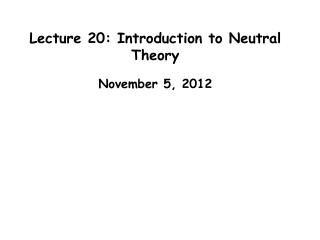
Lecture 20: Introduction to Neutral Theory November 5, 2012
Announcements Classes related to Population Genetics/Genomics next semester: BIOL 493S SPTP: Next Generation Biology CRN 18190, 1 credit, Tues 13:00-13:50 BIOL321 Total Science Experience Lab: Genomics Module, CRN 18084. W 13:00-15:50 2 credits (capstone) (special permission required, limit 12 students)
Last Time • Mutation introduction • Mutation-reversion equilibrium • Mutation and selection • Mutation and drift
Today • Introduction to neutral theory • Molecular clock • Expectations for allele frequency distributions under neutral theory
Classical-Balance • Fisher focused on the dynamics of allelic forms of genes, importance of selection in determining variation: argued that selection would quickly homogenize populations (Classical view) • Wright focused more on processes of genetic drift and gene flow, argued that diversity was likely to be quite high (Balance view) • Problem: no way to accurately assess level of genetic variation in populations! Morphological traits hide variation, or exaggerate it.
for m loci Molecular Markers • Emergence of enzyme electrophoresis in mid 1960’s revolutionized population genetics • Revealed unexpectedly high levels of genetic variation in natural populations • Classical school was wrong: purifying selection does not predominate • Initially tried to explain with Balancing Selection • Deleterious homozygotes create too much fitness burden
The rise of Neutral Theory • Abundant genetic variation exists, but perhaps not driven by balancing or diversifying selection: selectionists find a new foe: Neutralists! • Neutral Theory (1968): most genetic mutations are neutral with respect to each other • Deleterious mutations quickly eliminated • Advantageous mutations extremely rare • Most observed variation is selectively neutral • Drift predominates when s<1/(2N)
Infinite Alleles Model (Crow and Kimura Model) • Each mutation creates a completely new allele • Alleles are lost by drift and gained by mutation: a balance occurs • Is this realistic? • Average human protein contains about 300 amino acids (900 nucleotides) • Number of possible mutant forms of a gene: If all mutations are equally probable, what is the chance of getting same mutation twice?
Probability of sampling same allele twice Probability neither allele mutates Probability of sampling two alleles identical by descent due to inbreeding in ancestors Infinite Alleles Model (IAM: Crow and Kimura Model) • Homozygosity will be a function of mutation and probability of fixation of new mutants
Ignoring 2μ Ignoring μ2 Expected Heterozygosity with Mutation-Drift Equilibrium under IAM • At equilibrium ft = ft-1=feq • Previous equation reduces to: • Remembering that H=1-f: 4Neμ is called the population mutation rate, also referred to as θ
Expected Heterozygosity with Mutation-Drift Equilibrium under IAM • At equilibrium: set 4Neμ = θ • Remembering that H = 1-f:
Equilibrium Heterozygosity under IAM • Frequencies of individual alleles are constantly changing • Balance between loss and gain is maintained • 4Neμ>>1: mutation predominates, new mutants persist, H is high • 4Neμ<<1: drift dominates: new mutants quickly eliminated, H is low 2 Fraser et al. 2004 PNAS 102: 1968
Stepwise Mutation Model • Do all loci conform to Infinite Alleles Model? • Are mutations from one state to another equally probable? • Consider microsatellite loci: small insertions/deletions more likely than large ones? SMM: IAM:
Which should have higher produce He,the Infinite Alleles Model, or the Stepwise Mutation Model, given equal Ne and μ? Plug numbers into the equations to see how they behave. e.g, for Neμ= 1, He = 0.66 for SMM and 0.8 for IAM SMM: IAM:
Observed Avise 2004 Expected Heterozygosity Under Neutrality • Direct assessment of neutral theory based on expected heterozygosity if neutrality predominates (based on a given mutation model) • Allozymes show lower heterozygosity than expected under strict neutrality • Why?
Neutral Expectations and Microsatellite Evolution Autosomes • Comparison of Neμ(Θ) for 216 microsatellites on human X chromosome versus 5048 autosomal loci • Only 3 X chromosomes for every 4 autosomes in the population • Ne of X expected to be 25% less than Ne of autosomes: θX/θA=0.75 X Why is Θhigher for autosomes? X chromosome Correct model for microsatellite evolution is a combination of IAM and Stepwise • Observed ratio of ΘX/ΘA was 0.8 for Infinite Alleles Model and 0.71 for Stepwise model
Sequence Evolution • DNA or protein sequences in different taxa trace back to a common ancestral sequence • Divergence of neutral loci is a function of the combination of mutation and fixation by genetic drift • Sequence differences are an index of time since divergence
Molecular Clock • If neutrality prevails, nucleotide divergence between two sequences should be a function entirely of mutation rate Probability of creation of new alleles Probability of fixation of new alleles • Time since divergence should therefore be the reciprocal of the estimated mutation rate Expected Time Until Fixation of a New Mutation: Since μ is number of substitutions per unit time
Variation in Molecular Clock • So why are rates of substitution so different for different classes of genes? • If neutrality prevails, nucleotide divergence between two sequences should be a function entirely of mutation rate
The main power of neutral theory is it provides a theoretical expectation for genetic variation in the absence of selection.
Fate of Alleles in Mutation-Drift Balance Generations from birth to fixation Time between fixation events • Time to fixation of a new mutation is much longer than time to loss
Fate of Alleles in Mutation-Drift-Selection Balance Purifying Selection Which case will have the most alleles on average at any given time? What will this depend upon? Highest HE? Neutrality Balancing Selection/Overdominance
Assume you take a sample of 100 alleles from a large (but finite) population in mutation-drift equilibrium. What is the expected distribution of allele frequencies in your sample under neutrality and the Infinite Alleles Model? A. B. C. 10 8 6 Number of Alleles 4 2 2 2 2 4 4 4 6 6 6 8 8 8 10 10 10 Number of Observations of Allele
Black: Predicted from Neutral Theory White: Observed (hypothetical) Hartl and Clark 2007 Allele Frequency Distributions • Neutral theory allows a prediction of frequency distribution of alleles through process of birth and demise of alleles through time • Comparison of observed to expected distribution provides evidence of departure from Infinite Alleles model • Depends on f, effective population size, and mutation rate
Ewens Sampling Formula Population mutation rate: index of variability of population: Probability the i-th sampled allele is new given i alleles already sampled: Probability of sampling a new allele on the first sample: Probability of observing a new allele after sampling one allele: Probability of sampling a new allele on the third and fourth samples: . Expected number of different alleles (k) in a sample of 2N alleles is: Example: Expected number of alleles in a sample of 4: