Queuing in Operating Systems
Queuing in Operating Systems. References Probability, Statistics & Queuing Theory with Computer Science Applications (Allen - Academic Press Ltd) or any good queuing book. Lecture Objectives. Be able to recognize an operating system as a system of queues.

Queuing in Operating Systems
E N D
Presentation Transcript
Queuing in Operating Systems References Probability, Statistics & Queuing Theory with Computer Science Applications (Allen - Academic Press Ltd) or any good queuing book
Lecture Objectives • Be able to recognize an operating system as a system of queues. • Be able to calculate the steady state performance of a given fixed size queueing system. • Be able to show (calculate) the effect of a change on a simple queueing system caused by a change in arrival rate, service rate, system size, etc.
CPU Ready Queue Process Management • How do we manage them? • Keep track of states • Route efficiently • What do they look like to the system? • Randomly arriving tasks
OS as a System of Queues Realistic System job queue CPU ready queue I/O I/O queue wait queue time slice expired child executes fork child interrupt occurs wait for interrupt
Job Queue • What attributes are important in monitoring the Job Queue? • Random arrivals • Arrival rate? • Service time? • Queue size? • Distributions of arrivals and service times are key!!
Key is the distribution • If arrival rate is constant, solution is simple
Key is the distribution • If arrival rate is constant, solution is simple • (But this is not an accurate model)
Key is the distribution • If arrival rate is constant, solution is simple • (But this is not an accurate model) • If normal (Gaussian) distribution, better
Key is the distribution • If arrival rate is constant, solution is simple • (But this is not an accurate model) • If normal (Gaussian) distribution, better • Exponential model best
Management Objectives • Don't lose jobs • Don't delay jobs • Don't spend any more than needed
Book Store Example • 1 clerk • Short service line (3) • Average transaction rate (2/min) • Average arrival rate (1/min) 3 2 1 C Counter
Applications • CPU Jobs • I/O processing • File Access • Queue size • Delay • Loss
Terminology • Arrival rate () (inverse of mean inter-arrival time) • Service rate () (inverse of mean service time) • Assume steady state
State Transition diagram • 4 states (0--3) with arrivals and departures 0 1 2 3
State Transition diagram • 4 states (0--3) with arrivals and departures 0 1 2 3
0 1 2 3 State Transition diagram • 4 states (0--3) with arrivals and departures
0 1 2 3 State Transition diagram • 4 states (0--3) with arrivals and departures • Model assumptions - Markov • Memoryless • 1 event at a time
0 1 2 3 Balance Equations (State 0)
Balance Equations (State 0) 0 1 2 3
Balance equations • Assumes Steady State conditions • (system in balance) • 4 equations (1 is redundant)
0 1 Need 1 extra Equation • Additional Equation
Solve for P0 • Identify all Probabilities in terms of P0
Solve for P0 • Identify all Probabilities in terms of P0
Solve for P0 • Identify all Probabilities in terms of P0
What do the numbers mean? • Px is the probability of the system being in state x • There are x people waiting in line. • P0 is the probability that the system is empty • The clerk is idle • 1 - P0 is the probability that the system is busy • Utilization factor
Results • Idle => P0 = • Utilization = busy => 1 - P0 = • Throughput => * (1 - P0) = • Average queue size => 1 * P1 + 2*P2 + 3*P3 = • Lost customers => * P3 = • Little's Law => L = * W
Results • Idle => P0 = 8/15 • Utilization = busy => 1 - P0 = 7/15 • Throughput => * (1 - P0) = 14/15 • Average queue size => 1 * P1 + 2*P2 + 3*P3 = 11/15 • Lost customers => * P3 = 1/15 • Little's Law => L = * W = 11/15 = 1(W)==> 11/15
Arrival Rate = 1/min Service Rate = 2/min Calculate P0 Calculate throughput Clerk rate = $6/hr Profit = $3/book Calculate Net Profit Now add in Numbers
Application - • "Profit" from a CPU (or from a bookstore clerk) • Compare (higher throughput, but higher cost) • Cost $12/hr, Service rate 3/minute
Service Rate = 3/min Cost = $12 /hr P0 = 27/40 Utilization = 13/40 Throughput = 39/40 Profit = $2.73 /min Service Rate = 2/min Cost = $6 /hr P0 = 8/15 Utilization = 7/15 Throughput = 14/15 Profit = $2.70 /min Final Results
Extending the model • Different Queue Sizes • Multiple clerks • Multiple service times • Multiple arrival rates • Different distribution models.
Queuing ExtensionsInfinite queue (M/M/1) • P0 is dependent on allowable length of queue. • If the queue length is not constrained, then all probabilities change, affecting all other formulas.
Summary • Operating Systems can be abstracted as a system of queues. If we can understand the behavior of the queues, we can understand the system • Even though we assume that service and arrival rates are random, if they follow a generalized distribution, we can predict (in general) the behavior of the system
Questions • Given a queueing system of size 3 with a probability of being empty P0 = 27/65, an arrival rate of 2/min and a service rate of 3/min, what is the system throughput (rate at which customers move through the system)? • A) Please provide a state transition diagram for a queueing system that has a system size of 3. B) If the mean arrival rate is 3/min and the service rate is 4/min, what is the probability that a process will be lost due to overflow of the system? • A) Given a queueing system of size 3 with an arrival rate of 2/min and a service rate of 3/min, if we change the system size to 4, what effect will this have on the probability of losing a customer (go up, go down, stay the same)? B) Why?