Queuing Systems
690 likes | 1.01k Vues
Queuing Systems. Time-based versus event-based simulation Queuing systems as examples of discrete event systems The arrival process Performance measures Steady state Queuing theory: Birth and death processes. Time-Based Simulation.

Queuing Systems
E N D
Presentation Transcript
Queuing Systems • Time-based versus event-based simulation • Queuing systems as examples of discrete event systems • The arrival process • Performance measures • Steady state • Queuing theory: Birth and death processes
Time-Based Simulation • In time-based simulation the clock is incremented in steps of equal length. • We look at the system every minute, day, week, month, etc. • For a time-based simulation we do not need to know what happens within a single time step. All variables are updated at the end of the time step. • Typical example: inventory control (open spreadsheet Time Based Simulation.xls)
Event Based Simulation • Often systems change in a series of jumps (events) whose time of occurance is random • Examples: arrival or departure of customer / birth or death • Modelling assumption: • What happens between events is not important for the control of the system • A system whose evolution is driven by the occurance of events at random points in time is called a discrete event system
Event Based Control • The natural control mechanism for a discrete event simulation is event based: • For every class of events (arrival, departure, etc.) generate the next occurance time (possibly if an event (e.g. departure) cannot occur before another event (arrival) has taken place) • Advance the clock to the time of the next event • Update the system variables and list of next event times • Repeat until the simulation clock reaches a preset time • Flow charts are very helpful in setting up event based simulation programs
Entity Based Control • Entity based control: • An entity is a “player” who is processed through the system (e.g. a customer, an order) • When the entity enters the system, all necessary variables (e.g. arrival time, service time, arrival of next customer) are assigned to the entity using variables of past entities and RNGs • Control the number of entitites that pass through the system • Entity based control is particularly suitable for spreadsheet simulations • Open spreadsheet Event Based Simulation.xls
Queuing Systems • Time-based versus event-based simulation • Queuing systems as examples of discrete event systems • The arrival process • Performance measures • Steady state • Queuing theory: Birth and death processes
Queuing Systems • Events: • Arrivals and departures of customers • Customers balking or reneging • Customers moving from one queue to the next in a queuing network • etc. • Simple queuing system: • Customers arrive, queue up, are serviced, and depart. • Queuing networks: • Customers pass through a network of queues
The Queuing Paradigm • Characteristics of general queuing systems: • Entities flow through a system from one processing point to another • Some element of randomness • Main sources of randomness: • Arrival times • Specification of arriving entities • Processing times • Want to optimise the design and control of the system (e.g. manufacturing process) • Design variables, e.g., size, number and layout of processing points • Control variables, e.g., routing of entities through the system
Characteristics of simple queuing systems • The most important characteristics of a simple queuing system are the distributions of • interarrival times (times between arrivals of two consecutive customers) • service times (time for service of single customers). • It is often assumed that these random variables are (statistically) independent • Further important characteristics are the number of servers and the system capacity
Kendall’s notation • Simple queuing systems are conventionally labelled by U / V / s / / W • U and V denote the interarrival and service time distribution • most important abbreviations are D for deterministic, M for exponential and G for general (i.e. unspecified) distribution • s is the number of servers • is the system capacity (max. # customers in service and queue) • W is the queuing discipline (e.g. FIFO,LIFO,Priority based) • and W are optional with default values and W = FIFO
Kendall’s notation (continued) • Example: an M/M/s queue is a simple queuing system with exponential interarrival and service times, s servers, unlimited system capacity, and FIFO queuing discipline. • Tacit assumption when Kendall’s notation is used: • interarrival times are independent and identically distributed (i.i.d.) • service times are i.i.d. • interarrival and service times are independent
Uncertainty drivers • Main uncertainty drivers are interarrival times (times between the arrival of customers) and service times (times for service of a customer) • They control the evolution of the number N(t) of customers in the system at time t. • N(t) is called the state of the system at time t • Further uncertainties could be driving your model (e.g. amount of money spent by customers) • Frequent assumption: all random variables involved in the model are (statistically) independent
Arrival and service rates • The arrival rate is the expected number of arrivals per unit time (e.g. per hour) • The service rate is the expected number of customers that can be served by one of the servers per unit time • The expected service time per customer is 1/ • The expected time between two arrivals is 1/ • Arrival rate and service rate often depend on the time of the day, week, year,etc. (seasonal rates)
The utilization factor • Suppose a G/G/s queue • arrival rate , • service rate, • The utilization factor (or traffic intensity)is defined by s • Interpretation: is the fraction of time we expect the service facility to be busy (i.e. at least one of the servers to be busy) • If >1 then the queue “explodes” • What if <1 ?
An average case argument for <1 • Suppose s=1 (to make life easy) • If we simulate with interarrival times = average interarrival time (1/ ) service times = average service time (1/) then we obtain no queue • Ergo: the average queue length is zero? • Wrong: This is yet another example of the flaw of the averages • Let’s look at a spreadsheet model (open Waiting Time Versus Service Variance.xls)
Queuing Systems • Time-based versus event-based simulation • Queuing systems as examples of discrete event systems • The arrival process • Performance measures • Steady state • Queuing theory: Birth and death processes
The Role of the Exponential Distribution • What is a reasonable distribution for interarrival times? • What are typical properties of interarrival times? • An empirical observation: You have been sitting on a lake for half an hour trying to catch a fish - without success. Then your friend who is half an hour late as usual, joins you. Although you have already been sitting there for half an hour, your friend’s chances of catching a fish in the next 10 minutes are the same as yours.
The Lack-of-Memory Property “Probability of X>t+s, given X>s” (Conditional Probability) • The empirical observation can be formalized as P(X>t+s ¦ X>s)=P(Y>t), where X and Y are the time that elapses until you and your friend, resp., catch a fish. • Since both waiting times have the same distribution, i.e. P(X>t)=P(Y>t), we obtain P(X>t+s ¦ X>s)=P(X>t). • This property of a random variable is called the lack-of-memory property
Interarrival Time Distributions • The lack-of-memory property is typical for interarrival times, provided arrival rates are constant over time • Important Mathematical result: If a continuous random variable (with a continuous density function) has the lack-of-memory property then it is exponentially distributed • This mathematical result is the reason for the prevalence of the exponential distribution in queuing models
The exponential distribution • Parameter • Density function f(x)=e-x for x>0 and f(x)=0 for x • Cumulative distribution function F(x)=1-e-x for x>0 and F(x)=0 for x • Mean 1/ Standard deviation 1/ • Conclusion: If interarrival times have the lack-of-memory property then they are exponentially distributed with parameter arrival rate.
Spreadsheets We have seen before that, by using the inverse transform method, an exponentially distributed random variable with parameter l can be generated via =-ln(1-rand())/A1 where cell A1 contains the value l (Equivalently: -ln(rand())/A1 because “1-rand()” is a uniform RNG since rand() is a uniform RNG)
Service times • The lack-of-memory property is less typical for service times S. • However, in some situations the characteristics of the exponential distribution apply to the service time distribution • e.g. P(t St+t) decreases with t for every fixed t>0. • Drawback of exponential: mean = standard deviation • Whatever distribution is chosen for service or interarrival time, a goodness of fit test with sampled data should be used to check its validity • If in doubt use re-sampling from historical data
The minimum property Mathematical result: If X1,...,Xn are independent exponentially distributed random variables with parameters 1,...,n then X=min{X1,...,Xn} is exponentially distributed with parameter 1+...+ n .
Why is this important? • Example: If s independent exponentially distributed servers with service rates 1,..., s are busy then the time until the next service completion is exponentially distributed with parameter = 1+...+s. • Hence if the utilization factor is close to 100% (heavy traffic) then the behaviour of an M/M/s system with service rate approaches the behaviour of an M/M/1 system with service rate s
Disaggregation of arrival processes Mathematical result: If customers arrive with exponential interarrival times at rate and there are n types of customers with pi being the probability that a customer of type i arrives then the interarrival times of customers of type i are exponentially distributed with parameters i = pi
The Poisson Process • Let A(t) denote the number of customers that arrive in the time interval [0,t]. • Mathematical result: If the interarrival times are independent and exponentially distributed with parameter then A(t) has a Poisson distribution with parameter t, i.e. P(A(t)=n)=e-t((t)n/n!) • A(t) is called a Poisson arrival process • E[A(t)]=V[A(t)]= t (mean=variance)
Nonstationary Arrival Processes • One characteristic of a Poisson arrival process is P(A(t+t)=n+1 A(t)=n) t where the arrival rate is constant over time. • This is often an unrealistic assumption • A nonstationary (or nonhomogeneous) Poisson process allows the arrival rate to vary over time: P(A(t+t)=n+1 ¦ A(t)=n) tt. • The function (t) is called the arrival rate function
Generating nonstationary arrivals • Naïve implementation: Generate at time t arrival with rate l(t) • It’s better to use a thinning process: • Let max be an upper bound for the arrival rate function, i.e. (t) max for all t • Suppose the simulation clock has reached time t. • Generate an interarrival time x for the stationary process with arrival rate max • Increment clock to t+x • Accept arrival with probability (t)/max (i.e. generate a uniform RV u and neglect arrival if u> (t)/max ) • See spreadsheet Nonstationary Arrival Rates.xls
Queuing Systems • Time-based versus event-based simulation • Queuing systems as examples of discrete event systems • The arrival process • Performance measures • Steady state • Queuing theory: Birth and death processes
Performance Measures • Queuing models are often used to improve customer satisfaction • The main performance measures are queue length and waiting time • What do we mean by that? • Open spreadsheet Performance Measures.xls
What are we interested in? • The average queue length seen by the first N customers • is a random variable (changes with F9 key) • depends on N (moderate changes as N gets large) • Mathematically: Interested in the distribution of the average as N tends to (long run average) • Practically: Interested in the distribution for large N (simulation)
Average waiting time • Can simulate waiting times for each customer • Can simulate average waiting time of first N customers • Average waiting time of first N customers • is a random variable • depends on N (becomes smoother as N grows)
Queuing Systems • Time-based versus event-based simulation • Queuing systems as examples of discrete event systems • The arrival process • Performance measures • Steady state • Queuing theory: Birth and death processes
Focus on simple queuing systems • Process: Customers arrive -> queue up -> are served (FIFO) -> leave • Characteristics • Interarrival time • Service time • Number of servers • System capacity
Steady State • The stateN(t) of a queuing system at time t is the number of customers in the system (i.e. in the queue or in service) at time t • The system is said to be in steady state if P(N(t)=n) does not change with t any more. • Simple queuing system reaches steady state only if <1 • Let’s look at a spreadsheet… (open Steady State.xls)
Steady State Distribution • If the system is in steady state then the distribution characterized by the probability mass function pn=P(N=n) is called the steady state distribution • Mathematically, pn is defined to be the limit of P(N(t)=n) as t tends to infinity (provided the limits exist and the pn add up to 1). • In simulation experiments it is often advisable to allow for a run-in time before measurements (e.g. waiting times) are taken in order to allow the system to reach steady state.
Average Queue Length • Expected number of customers in the system (in steady state) is L=1p1+2p2+3p3+4p4+... • Expected queue length of an s-server system (in steady state) is Lq = 1ps+1+2ps+2+3ps+3+4ps+4+...
Average Waiting Time • W: average waiting time (until service completion) for a customer in the system (in steady state) • Wq: average waiting time for a customer in the queue • Relationship: W=Wq+1/ • Little’s formula clarifies the relation between Wq and Lq….
Little’s Formula • In steady state a newly arriving customer expects to see a queue of length Lq • She is expected to be in the queue for Wqtime units • During these Wq time units one expects that Wq new customers arrive • So the queue length is expected to be Wqwhen the customer leaves the queue • In steady state the expected queue length when a customer arrives is the same as the expected queue length when she leaves the queue; hence we obtain Lq =Wq
Queuing Systems • Time-based versus event-based simulation • Queuing systems as examples of discrete event systems • The arrival process • Performance measures • Steady state • Queuing theory: Birth and death processes
Queuing Theory Traditional queuing theory is concerned with obtaining closed form solutions for steady state probabilities pn=P(N=n) or the performance measures L,Lq,W, and Wq for simple queuing systems.
The Birth and Death Process • A simple queuing system is a special case of a birth and death process • “Birth” = “arrival of customer” • “Death” = “departure of customer” • State N(t) is the size of a population at time t • Births and Deaths happen randomly with rates possibly depending on the size of the population.
Assumptions for B & D Process • Given time t and state N(t)=n, the probability distribution of the remaining time until the next birth is exponential with parameter n. • Given time t and state N(t)=n>0, the probability distribution of the remaining time until the next death is exponential with parameter n. • The random variables of the above assumptions are mutually independent. • The process is in steady state, i.e. P(N(t)=n) is independent of the time t.
The Balance Equation • At any time the next state transition is either from n to n+1 or from n to n-1, depending on whether a birth or a death occurs next. • Define Enand Ln to be the rate (average number of events per unit time) at which the system enters and leaves state n, respectively. • Balance equation: En= Ln Rate in = Rate out
Steady State Probabilities • Recall that pn=P(N=n). • Notice that pn can be interpreted as the proportion of time the process is in state n • Idea: Express En and Ln in terms of steady state probabilities pn and use balance equation to calculate pn.
A Formula for E0 • The process can only enter state 0 from state 1 • p1 is the proportion of time the process is in state 1 • is the rate at which the process enters state 0 from state 1 • Hence E0= p1
Further formulas Similar arguments show that L0= p0 En=pn-1n-1+pn+1n+1 Ln=pn (n+n)
The Balance Equation Revisited • Using the balance equation E0=L0 we obtain p1= (0/1)p0 • Using the balance equations En=Ln for n>0 we further obtain pn+1= (n/n+1)pn +(/n+1)(npn -n-1pn-1) • Given p0, we can calculate pn recursively as pn= cnp0 with cn= (01...n-1(12...n
