Layout
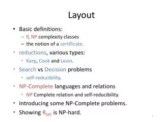
Layout. Basic definitions: P , NP complexity classes the notion of a certificate . reductions , various types: Karp , Cook and Levin . Search vs Decision problems self-reducibility . NP-Complete languages and relations NP Complete relation and self-reducibility.

Layout
E N D
Presentation Transcript
Layout • Basic definitions: • P, NP complexity classes • the notion of a certificate. • reductions, various types: • Karp, Cook and Levin. • SearchvsDecision problems • self-reducibility. • NP-Complete languages and relations • NP Complete relation and self-reducibility. • Introducing some NP-Complete problems. • Showing RSAT is NP-hard.
The P, NP complexity classes Def:ADecision problem for a language L {0,1}*is to decide whether a given string x belongs to the language L. Def:P is the class of languages (decision problems) that can be recognized by a deterministic polynomial time Turing machine. Def:NP is the class of languages that can be recognized by a non-deterministic polynomial-time Turing-machine.
Polynomially Verifiable Relations Def: A binary relation Ris polynomially bounded if:(x,y) R |y| |x|o(1) Def:R is polynomial-time-decidable if the corresponding languageLR = { (x,y) : (x,y) R }is in P. Def: A relation that is both polynomially-bounded & polynomial-time-decidable is polynomially-verifiable.
NP – Alternative Definition Def:L is an NP language if there is a polynomially-verifiable relation RLs.t.X L w for which (x,w) RL w is a witness or a certificate. Given a witness, membership can be verified in polynomial time. P=NP implies: witness can be found efficiently
The NP game The notion of a certificate can be thought of a game between a prover and a verifier Given input X The all powerful prover sends a certificate for membership of X Which the verifier can validate efficiently prover verifier
NDTM PolyVerRel 1.2.1 • Assume ML is a non-deterministic TM that decides L within PL( |x| ) steps • Let RL be the set of all pairs (x,y) s.t. • x is an input to ML • Y is an accepting, legal computation of MLon x • RL is polynomially-verifiable • XL a computation y s.t. (x,y) RL
PolyVerRel NDTM • Let RL be the relation for L, decided by a deterministic TM M*L • Def a non-deterministic TM ML: • Guess y of proper polynomial size • Call M*L to checkif (x,y) RL • Accept x if M*L accepts (x,y) • ML is a non-deterministic TM for L
Search Problems • Def: A search problem over a binary relation R finds, given x, a string y s.t. (x,y) R. • Given a polynomially-verifiable relation R, define:L(R) = { x : y s.t. (x,y) R } Clearly, finding a solution can only be harder than just deciding whether it exists. Note: NP = { L(R) : R is polynomially-verifiable }
Example Problem:3-coloring graphs Instance: An undirected graph G=(V,E) Corresponding relation: R3COL = { (G,) : is a legal 3-coloring of G } Decision problem: decide the language L(R3COL), namely whether G is 3-colorable. Search problem: find a 3-coloring of G.
Reductions 2.1 • The purpose of a reductionis to show that some problem is at least as hard as some other problem. • If problem Areduces to problem B, then solving B implies solving A. B is at least as hard as A, denoted A B
Cook Reduction Def: An oraclefor a problem is a magical apparatus that, given an input x to , returns (x) in a single step. Def: ACook reductionfrom problem 1to problem 2is a polynomial-time TM for solving 1 on input x utilizing an oracle for 2.Denoted1 cook 2.
L2 f L2 L2 L1 L1 Karp Reduction Def: AKarp reductionof L1to L2 is a polynomial-time--computable function f s.t.x L1 f(x) L2 f(x) x f(x)
Solve 1 I/o 2 oracle Karp vs. Cook reductions Cook reduction allows calling the oracle polynomially many times Karp reduction allows only one call to the oracle, and only at the end of the computation. • Cook reduction is stronger: given Karp reduction f, • On input x compute the value f(x). • Present f(x) to the oracle, and output its answer. • There are (few) examples where a Cook reduction is known, while a Karp reduction is unknown.
Note: A Levin reduction implies Cook / Karp reductions of the corresponding search / decision problems. Levin Reduction 2.1 Def: aLevin reductionfrom R1to R2is 3 poly-time-computable functions f,g,h s.t. • x L(R1) f(x) L(R2) • (x,y) R1 ( f(x), g(x,y) ) R2 • ( f(x),z ) R2 ( x, h(x,z) ) R1 f translates inputs of the first problem to inputs of the second problem, g & h transform certificates of one to the other.
Properties of Reductions 2.1 Claim: All reductions are transitive:A reduces to B, B to C A reduces to C Claim:Cook reduction preserves poly-time-computability Proof: assume 1Cook-reduces to the poly-time-comp problem 2, and M is the reduction algorithm. • 2-oracle can be simulated by a poly-time TM • Replacing oracle queries in M by the simulation - we get a poly-time TM that solves 1. So do Karp & Levin reductions
Search vs. Decision Problems 1.4 Recall: for poly-time verifiable relationR,L(R) = { x : y s.t. (x,y) R } Def: A relation R is called self-reducibleif solving the search problem for R is Cook-reducible to deciding the language L(R). The search problem can be solved using the decision problem
Note: Self-reducibility is a property of a relation, not a language.[There are many relations R for which SAT = L(R).] An Example: 3-SAT Input: A CNF formula with n variables. Task: find : {1,..,N} {0,1} such that ( (1), …, (n) ) = True Corresponding relation: RSAT = { (, ) : ( (1), …, (n) ) = T } SAT = L(RSAT)
RSAT 1.4.1 Thm: RsatisSelf-Reducible. Proof:Assuming an oracle O for the language SAT = L(RSAT). solving the search problem: Query O whether SAT. If not - stop. • For k := 1 to n: • K (xk+1, .., xn) := ( 1, .., k-1,1, xk+1,.., xn) • If k SAT (Query O), k = 1else k = 0. • (1)=1, …, (n)=n satisfies ! formula obtained by replacingx1, ..,xk with1, .., k-1,1
SAT oracle Self-reducibility of SAT Given:( x y) ( x z) Yes ( x y) ( x z) No x = 1: (1 y) (1 z) y = 1: ( 1 1) ( 1 z) y = 1: ( 1 1) ( 1 z) y = 0: ( 1 0) ( 1 z) z = 1: ( 1 0) ( 1 1)
Another Example: GI Graph Isomorphism: given two (simple) graphs, are they isomorphic? Natural relation: RGI contains all ( (G1,G2),)s.t. is an isomorphism between G1 and G2. Unlike SAT, GI is not known to be NP-Complete in fact GI is unlikely to be NP-hard, as we’ll see later in the course
RGI 1.4.2 Thm:RGI is Self-Reducible. Proof: construct piecemeal, 1 vertex at a timecheck if u G1 can be mapped by to v G2: • Connect both v and u to new n leaf-verticesto obtain 2 new graphs, G’1 & G’2 • If G’1 isomorphic to G’2 - u must be mapped to v • Iterating this - deleting matching vertices - determines the isomorphism, a vertex at a time u and v are distinguished from other vertices so any isomorphism must map u to v
Non Self-Reducibility • There are many non-self-reducible relations, but it is hard to find an NP language, whose “natural” relation is non-self-reducible. • LCOMP = { N : N = n1 n2 } is poly- time decidable via a randomized algorithm. • The natural choice is RCOMP = { ( N, (n1,n2) ) : N = n1 n2 } • It is widely believed the search of RCOMP is not poly-time-comp (factoring), which would imply it is not self-reducible (by a random algorithm) deterministic!
NP-completeness Def: A language L is NP-Complete if: 1. LNP. 2. L’NP: L’KarpL . Generalize: L’CookL • Def: A relation R is NP-Complete if: • 1. L(R)NP. • 2. R’ s.t. L(R’)NP: R’LevinR.
NP-completeness & Self-Reducibility 2.2 Thm: For every relation R, R is NP-Complete R is self-reducible. Proof: Let R be an NP-complete relation. RSAT is NP-hard under Levin reduction (to be proven later), namely, there is a Levin reduction (f,g,h) from R to RSAT Since R is NP-complete, there exists aKarp reduction k from SAT to L(R).
NP-completeness & Self-Reducibility • Proof (continue): analgorithm that finds y s.t. (x,y)R,using the Levin & karp reductions: • Query L(R)’s oracle whether xL(R) • If “no”, announce: xL(R) • If “yes”, translate x into a CNF formula f(x)[using Levin’s f function] • Compute a satisfying assignment (1,…,n) for • Translate (1,…,n) to a witness y=h(x, (1,…,n))[Using Levin’s h function] xL(R) f(x)L(RSAT) show later f(x,z) L(RSAT) (x,h(x,z))L(R)
NP-completeness & Self-reducibility • Proof (continue):given a partial assignment (1,…,i),compute a satisfying assignment (1,…,n) for , • Trying to assign xi+1: • check L(R)’s oracle to see if(1,…,i,1,xi+2,…, xn) is satisfiable[By translating the CNF formula (1,…,i,1,xi+2,…, xn) to the language L(R), using the Karp function k] • If the oracle answers “yes” assign i+1, otherwise assign i+1 • Iterate until in. SATKarpL(R) and since L(R) is NP-complete SAT k()L(R) same as in self-reducibility of SAT. instead of SAT’s oracle, use L(R)’s oracle
NP-completeness & Self-reducibility L oracle SAT L Given:( x y) ( x z) ( x y) ( x z) x = 1: (1 y) (1 z) y = 1: ( 1 1) ( 1 z) y = 1: ( 1 1) ( 1 z) y = 0: ( 1 0) ( 1 z) Yes No z = 1: ( 1 0) ( 1 1)
Bounded-Halting 2.3 Two Equivalent Definitions: BH { <M>,x,1t | <M> is the description of a non-deterministicTM that accepts input x within t steps. } BH { <M>,x,1t | <M> is the description of a deterministic TM, and y s.t. |y||x|O(1)and M accepts (x,y) within t steps }
Note: The length of y is bounded by t, therefore it is polynomial in the length of the input <M>,x,1t . Bounded-Halting Cont. Def:Bounded-Halting Relation RBH { (<M>,x,1t , y)|<M> is the description of a deterministic machine, which accepts input (x,y) within t steps}
Bounded-Halting is NP-Complete Claim:BH is NP-Complete. Proof: • BHNP (immediate from definition) • Any L in NP, Karp-reduces to BH:Let L be in NP, then: • There exists a poly-time verifiable witness-relation RL, recognized by ML. • ML accepts every (x,y) in p(|x|) steps • The reduction transforms x toML,x,1p(|x|)
Note:The reduction can be transformed into Levin reduction of RL to RBH with the identity function supplying the two missing functions. Bounded-Halting is NP-complete Proof (continue): XL Exists a polynomially bounded witness y suchthat (x,y)RL Exists a polynomial time computation of MLaccepting (x,y) ML,x,1p(|x|) BH (x,y) ( M,x,1t ,y)
Xi Out 1 Circuit-Satisfiability 2.4 Def: a circuit is a directed acyclic graph G=(V,E) with vertices labeled output,,,,x1,…, xm, s.t. • A vertex labeled xihas in-degree 0 • A vertex labeled 0 (or 1) has in-degree 0 • The in-degree of vertices labeled , is 2 (bounded fan-in) • A vertex labeled has in-degree 1 • a single sink (of out-degree 0), of in-degree 1, labeled “output”
Circuit-Satisfiability Given an assignment mto the variables x1,…,xm, C() will denote the value of the circuit’s output Def:Circuit-Satisfiabilty CS {circuit C : exists s.t. C()=1} RCS {(C, ) : C()=1} The value is defined by setting the value of each vertex to the natural value imposed by the Boolean operation it is labeled by
CS is NP-complete 2.4,2.6 Claim:CSisNP-Complete. Proof: • CSNP • RCS is polynomialy-bounded: the witness is an assignment - it has one bit for each xi • Given a pair (C, ) evaluating one gate takes O(1) steps, therefore total evaluation time is polynomial in |C|.
CS is NP-complete Proof (continue): • CS is NP-hard (show a reduction from BH): Given M,x,1t the computation of M can be fully described by a ttmatrix in which entry (i,j) is: • The content of cell j at time i (constant) • An indicator to whether the head is on cell j at time i (1 bit). • In case the head is indeed there: the state of the machine ( O(log |M|) ). Each row of the matrix corresponds to a configuration of the machine
CS is NP-complete Proof (continue): • The transition between following configurations can be simulated by a series of t circuits Ctas shown later. • The reduction constructs a circuit C’ from the t t Ctcircuits, where the ith series is the input of the i+1 series. • The input to the circuit is built of |x| vertices corresponding to the input x, and t-|x| “variable vertices”. • Finally, we add to C’ the ability to identify that a certain configuration has reached accepting state, so that the circuit will output 1. • It is shown that the whole circuit can be built using O(n5) gates.
Symbol Head indicator Log |M| state bits Symbol Head indicator Log |M| state bits Symbol Head indicator Log |M| state bits The circuit Ct • The j’th triple in the i’th configuration, is determined by the j-1, j, j+1 triples in the i-1 configuration. This can be described by boolean functions implemented by Ct. J-1 Symbol Head indicator Ct J Log |M| state bits J+1 I’th-1 configurtion I’th configuration It is shown that Ctcan be described in O(n3) gates
CS is NP-complete Proof (continue): • The accepting states can be encoded into a Boolean function, which will return 1, on input an accepting state. The output of the entire circuit is an OR over all the state outputs of all Ct circuits. This can be described by O(n2 log n) gates.
RSAT is NP-hard 2.5 Claim: RSATis NP-hard under Levin reduction. Proof: Since Circuit-satisfiability is NP-Complete it suffices to show a reduction from RCS to RSAT: The reduction maps a circuit C to a CNF formula C, and an input y for the circuit to an assignment y’*to the formula and vice versa.
RSAT is NP-hard Proof (continue): Mapping circuit C to CNF formula C • Every vertex of the circuit-graph is mapped into a variable. • For every such variable Vi we define a CNF formula ithat forces the variable to have the same value as the gate represented by Vi • We define c 1 … n
RSAT is NP-hard • Proof (continue): mapping a gate to a formula: • For a vertex vwith an in-edge from u:i (v, u) (u v) (u v) • For a vertexv with in-edges from u, w:i (v, u, w) (u w v) (u w v) (u w v) (u w v) • For a vertex v with in-edges from u, w:i (v, u, w) (u w v) (u w v) (u w v) (u w v) • For the vertex marked output with an in-edge from u:output(u) u
RSAT is NP-hard Proof (continue): • CCS cSAT: given an assignment to c it’s easy to construct an assignment to C, and vice versa • Note: The reduction is poly-time - the size of the CNF formula c is linear in the size of C, therefore, it can be constructed in polynomial time