Mastering Integration Techniques: Substitution, Parts, Definite Integrals
580 likes | 767 Vues
Learn how to apply integration by substitution and parts, evaluate definite integrals, approximate integrals, and explore integral applications. Practice examples and step-by-step solutions provided.

Mastering Integration Techniques: Substitution, Parts, Definite Integrals
E N D
Presentation Transcript
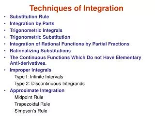
Chapter Outline • Integration by Substitution • Integration by Parts • Evaluation of Definite Integrals • Approximation of Definite Integrals • Some Applications of the Integral • Improper Integrals
§9.1 Integration by Substitution
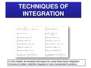
Section Outline • Differentiation and Integration Formulas • Integration by Substitution • Using Integration by Substitution
Integration by Substitution If u = g(x), then
Using Integration by Substitution EXAMPLE Determine the integral by making an appropriate substitution. SOLUTION Let u = x2 + 2x + 3, so that . That is, Therefore, And so we have Rewrite in terms of u. Bring the factor 1/2 outside. Integrate.
Using Integration by Substitution CONTINUED Replace u with x2 + 2x + 3.
Using Integration by Substitution EXAMPLE Determine the integral by making an appropriate substitution. SOLUTION Let u = 1/x + 2, so that . Therefore, And so we have Rearrange factors. Rewrite in terms of u. Integrate. Rewrite u as 1/x + 2.
Using Integration by Substitution EXAMPLE Determine the integral by making an appropriate substitution. SOLUTION Let u = cos2x, so that . Therefore, And so we have Rearrange factors. Rewrite in terms of u. Integrate. Rewrite u as cos2x.
§9.2 Integration by Parts
Section Outline • Integration by Parts • Using Integration by Parts
Integration by Parts G(x) is an antiderivative of g(x).
Using Integration by Parts EXAMPLE Evaluate. SOLUTION Our calculations can be set up as follows: Differentiate Integrate Then
Using Integration by Parts CONTINUED
Using Integration by Parts EXAMPLE Evaluate. SOLUTION Our calculations can be set up as follows: Then Notice that the resultant integral cannot yet be solved using conventional methods. Therefore, we will attempt to use integration by parts again.
Using Integration by Parts CONTINUED Our calculations can be set up as follows: Then Therefore, we have
Using Integration by Parts EXAMPLE Evaluate. SOLUTION Our calculations can be set up as follows: Then
Using Integration by Parts CONTINUED
§9.3 Evaluation of Definite Integrals
Section Outline • The Definite Integral • Evaluating Definite Integrals • Change of Limits Rule • Finding the Area Under a Curve • Integration by Parts and Definite Integrals
The Definite Integral where F΄(x) = f(x).
Evaluating Definite Integrals EXAMPLE Evaluate. SOLUTION First let u = 1 + 2x and therefore du = 2dx. So, we have
Evaluating Definite Integrals CONTINUED Consequently,
Using the Change of Limits Rule EXAMPLE Evaluate using the Change of Limits Rule. SOLUTION First let u = 1 + 2x and therefore du = 2dx. When x = 0 we have u = 1 + 2(0) = 1. And when x = 1, u = 1 + 2(1) = 3. Thus
Finding the Area Under a Curve EXAMPLE Find the area of the shaded region. SOLUTION To find the area of the shaded region, we will integrate the given function. But we must know what our limits of integration will be. Therefore, we must determine the three x-intercepts of the function. This is the given function.
Finding the Area Under a Curve CONTINUED Replace y with 0 to find the x-intercepts. Set each factor equal to 0. Solve for x. Therefore, the left-most region (above the x-axis) starts at x = -3 and ends at x = 0. The right-most region (below the x-axis) starts at x = 0 and ends at x = 3. So, to find the area in the shaded regions, we will use the following. Now let’s find an antiderivative for both integrals. We will use u = 9 – x2 and du = -2xdx.
Finding the Area Under a Curve CONTINUED Now we solve for the area.
Finding the Area Under a Curve CONTINUED
Integration by Parts & Definite Integrals EXAMPLE Evaluate. SOLUTION To solve this integral, we will need integration by parts. Our calculations can be set up as follows: Then
Integration by Parts & Definite Integrals CONTINUED Therefore, we have
§9.4 Approximation of Definite Integrals
Section Outline • The Midpoint Rule • The Trapezoidal Rule • Simpson’s Rule • Error Analysis
Using the Midpoint Rule EXAMPLE Approximate the following integral by the midpoint rule. SOLUTION We have Δx = (b – a)/n = (4 – 1)/3 = 1. The endpoints of the four subintervals begin at a = 1 and are spaced 1 unit apart. The first midpoint is at a + Δx/2 = 1.5. The midpoints are also spaced 1 unit apart. According to the midpoint rule, the integral is approximately equal to
Using the Trapezoidal Rule EXAMPLE Approximate the following integral by the trapezoidal rule. SOLUTION As in the last example, Δx = 1 and the endpoints of the subintervals are a0 = 1, a1 = 2, a2 = 3, and a3 = 4. The trapezoidal rule gives
Using Simpson’s Rule EXAMPLE Approximate the following integral by Simpson’s rule. SOLUTION As in the last example, Δx = 1 and the endpoints of the subintervals are a0 = 1, a1 = 2, a2 = 3, and a3 = 4. Simpson’s rule gives NOTE: Although this happens to be the exact answer, remember that Simpson’s Rule is still just an approximation and therefore it generally yields only an estimate of the exact answer, not the exact answer itself.
Using Error Analysis EXAMPLE Obtain a bound on the error of using the midpoint rule with n = 3 to approximate SOLUTION Here a = 1, b = 4, and f(x) = (2x – 3)3. Differentiating twice, we find that How large could | f΄΄(x)| be if x satisfies 1 ≤ x ≤ 4? Since the function 48x – 72 is clearly increasing on the interval from 1 to 4 (in fact, it’s increasing everywhere), its greatest value occurs at x = 4. Therefore, its greatest value is
Using Error Analysis CONTINUED so we may take A = 120 in the preceding theorem. The error of approximation using the midpoint rule is at most NOTE: We have hitherto determined that the exact value of this integral is 78 and that the midpoint approximation for it (using n = 3) is 72. Therefore, this approximation was in error by 78 – 72 = 6. Our result in this exercise says that our midpoint approximation error should be no greater than 15. Since 6 is no greater than 15, this result suggests that our midpoint approximation was done correctly.
§9.5 Some Applications of the Integral
Section Outline • The Riemann Sum • Interest Compounded Continuously • Continuous Stream of Income • Population in a Ring
The Riemann Sum Δx = (b – a)/n, t1, t2, …., tn are selected points from a partition [a, b].
Continuous Stream of Income EXAMPLE Find the present value of a stream of earnings generated over the next 2 years at the rate of 50 + 7t thousand dollars per year at time t, assuming a 10% interest rate. SOLUTION Using the theorem above, we have K(t) = 50 + 7t, r = 0.06, T1 = 0 and T2 = 2. So, we have To evaluate, we will need to rewrite the integral as and then evaluate the first integral directly and the second using integration by parts. Upon doing this, we have
Continuous Stream of Income CONTINUED Now we evaluate the integral. So the present value of the described stream of earnings is $102.90.