Download
1 / 57
580 likes | 735 Vues
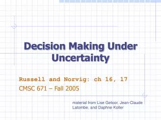
Decision Making Under Uncertainty. Russell and Norvig: ch 16, 17 CMSC421 – Fall 2003. material from Jean-Claude Latombe, and Daphne Koller. sensors. environment. ?. agent. actuators. Utility-Based Agent. ?. ?. a. a. b. b. c. c. {a(p a ),b(p b ),c(p c )}

E N D
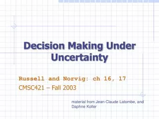
Decision Making Under Uncertainty Russell and Norvig: ch 16, 17 CMSC421 – Fall 2003 material from Jean-Claude Latombe, and Daphne Koller
sensors environment ? agent actuators Utility-Based Agent
? ? a a b b c c • {a(pa),b(pb),c(pc)} • decision that maximizes expected utility value Non-deterministic vs. Probabilistic Uncertainty • {a,b,c} • decision that is best for worst case Non-deterministic model Probabilistic model ~ Adversarial search
Expected Utility • Random variable X with n values x1,…,xn and distribution (p1,…,pn)E.g.: X is the state reached after doing an action A under uncertainty • Function U of XE.g., U is the utility of a state • The expected utility of A is EU[A] = Si=1,…,n p(xi|A)U(xi)
s0 A1 s1 s2 s3 0.2 0.7 0.1 100 50 70 One State/One Action Example U(S0) = 100 x 0.2 + 50 x 0.7 + 70 x 0.1 = 20 + 35 + 7 = 62
s0 A1 A2 s1 s2 s3 s4 0.2 0.7 0.2 0.1 0.8 100 50 70 One State/Two Actions Example • U1(S0) = 62 • U2(S0) = 74 • U(S0) = max{U1(S0),U2(S0)} • = 74 80
MEU Principle • rational agent should choose the action that maximizes agent’s expected utility • this is the basis of the field of decision theory • normative criterion for rational choice of action AI is Solved!!!
Not quite… • Must have complete model of: • Actions • Utilities • States • Even if you have a complete model, will be computationally intractable • In fact, a truly rational agent takes into account the utility of reasoning as well---bounded rationality • Nevertheless, great progress has been made in this area recently, and we are able to solve much more complex decision theoretic problems than ever before
We’ll look at • Decision Theoretic Planning • Simple decision making (ch. 16) • Sequential decision making (ch. 17)
Decision Networks • Extend BNs to handle actions and utilities • Also called Influence diagrams • Make use of BN inference • Can do Value of Information calculations
Decision Networks cont. • Chance nodes: random variables, as in BNs • Decision nodes: actions that decision maker can take • Utility/value nodes: the utility of the outcome state.
Umbrella Network take/don’t take umbrella P(rain) = 0.4 weather Lug umbrella forecast P(lug|take) = 1.0 P(~lug|~take)=1.0 happiness f w p(f|w) sunny rain 0.3 rainy rain 0.7 sunny no rain 0.8 rainy no rain 0.2 U(lug,rain) = -25 U(lug,~rain) = 0 U(~lug, rain) = -100 U(~lug, ~rain) = 100
Evaluating Decision Networks • Set the evidence variables for current state • For each possible value of the decision node: • Set decision node to that value • Calculate the posterior probability of the parent nodes of the utility node, using BN inference • Calculate the resulting utility for action • return the action with the highest utility
the value of the new best action (after new evidence E’ is obtained): the value of information for E’ is: Value of Information (VOI) • suppose agent’s current knowledge is E. The value of the current best action is
Sequential Decision Making • Finite Horizon • Infinite Horizon
Simple Robot Navigation Problem • In each state, the possible actions are U, D, R, and L
Probabilistic Transition Model • In each state, the possible actions are U, D, R, and L • The effect of U is as follows (transition model): • With probability 0.8 the robot moves up one square (if the robot is already in the top row, then it does not move)
Probabilistic Transition Model • In each state, the possible actions are U, D, R, and L • The effect of U is as follows (transition model): • With probability 0.8 the robot moves up one square (if the robot is already in the top row, then it does not move) • With probability 0.1 the robot moves right one square (if the robot is already in the rightmost row, then it does not move)
Probabilistic Transition Model • In each state, the possible actions are U, D, R, and L • The effect of U is as follows (transition model): • With probability 0.8 the robot moves up one square (if the robot is already in the top row, then it does not move) • With probability 0.1 the robot moves right one square (if the robot is already in the rightmost row, then it does not move) • With probability 0.1 the robot moves left one square (if the robot is already in the leftmost row, then it does not move)
Markov Property The transition properties depend only on the current state, not on previous history (how that state was reached)
Sequence of Actions [3,2] 3 2 1 1 2 3 4 • Planned sequence of actions: (U, R)
[3,2] [3,2] [3,3] [4,2] Sequence of Actions 3 2 1 1 2 3 4 • Planned sequence of actions: (U, R) • U is executed
[3,2] [3,2] [3,3] [4,2] [3,1] [3,2] [3,3] [4,1] [4,2] [4,3] Histories 3 2 1 1 2 3 4 • Planned sequence of actions: (U, R) • U has been executed • R is executed • There are 9 possible sequences of states – called histories – and 6 possible final states for the robot!
Probability of Reaching the Goal 3 Note importance of Markov property in this derivation 2 1 1 2 3 4 • P([4,3] | (U,R).[3,2]) = • P([4,3] | R.[3,3]) x P([3,3] | U.[3,2]) + P([4,3] | R.[4,2]) x P([4,2] | U.[3,2]) • P([4,3] | R.[3,3]) = 0.8 • P([4,3] | R.[4,2]) = 0.1 • P([3,3] | U.[3,2]) = 0.8 • P([4,2] | U.[3,2]) = 0.1 • P([4,3] | (U,R).[3,2]) = 0.65
3 +1 2 -1 1 1 2 3 4 Utility Function • [4,3] provides power supply • [4,2] is a sand area from which the robot cannot escape
3 +1 2 -1 1 1 2 3 4 Utility Function • [4,3] provides power supply • [4,2] is a sand area from which the robot cannot escape • The robot needs to recharge its batteries
3 +1 2 -1 1 1 2 3 4 Utility Function • [4,3] provides power supply • [4,2] is a sand area from which the robot cannot escape • The robot needs to recharge its batteries • [4,3] or [4,2] are terminal states
3 +1 2 -1 1 1 2 3 4 Utility of a History • [4,3] provides power supply • [4,2] is a sand area from which the robot cannot escape • The robot needs to recharge its batteries • [4,3] or [4,2] are terminal states • The utility of a history is defined by the utility of the last state (+1 or –1) minus n/25, where n is the number of moves
Utility of an Action Sequence +1 3 -1 2 1 1 2 3 4 • Consider the action sequence (U,R) from [3,2]
[3,2] [3,2] [3,3] [4,2] [3,1] [3,2] [3,3] [4,1] [4,2] [4,3] Utility of an Action Sequence +1 3 -1 2 1 1 2 3 4 • Consider the action sequence (U,R) from [3,2] • A run produces one among 7 possible histories, each with some probability
[3,2] [3,2] [3,3] [4,2] [3,1] [3,2] [3,3] [4,1] [4,2] [4,3] Utility of an Action Sequence +1 3 -1 2 1 1 2 3 4 • Consider the action sequence (U,R) from [3,2] • A run produces one among 7 possible histories, each with some probability • The utility of the sequence is the expected utility of the histories:U = ShUhP(h)
[3,2] [3,2] [3,3] [4,2] [3,1] [3,2] [3,3] [4,1] [4,2] [4,3] Optimal Action Sequence +1 3 -1 2 1 1 2 3 4 • Consider the action sequence (U,R) from [3,2] • A run produces one among 7 possible histories, each with some probability • The utility of the sequence is the expected utility of the histories • The optimal sequence is the one with maximal utility
[3,2] [3,2] [3,3] [4,2] [3,1] [3,2] [3,3] [4,1] [4,2] [4,3] only if the sequence is executed blindly! Optimal Action Sequence +1 3 -1 2 1 1 2 3 4 • Consider the action sequence (U,R) from [3,2] • A run produces one among 7 possible histories, each with some probability • The utility of the sequence is the expected utility of the histories • The optimal sequence is the one with maximal utility • But is the optimal action sequence what we want to compute?
Accessible or observable state Reactive Agent Algorithm Repeat: • s sensed state • If s is terminal then exit • a choose action (given s) • Perform a
+1 3 -1 2 1 1 2 3 4 Policy (Reactive/Closed-Loop Strategy) • A policy P is a complete mapping from states to actions
Reactive Agent Algorithm Repeat: • s sensed state • If s is terminal then exit • aP(s) • Perform a
Note that [3,2] is a “dangerous” state that the optimal policy tries to avoid Makes sense because of Markov property Optimal Policy +1 3 -1 2 1 1 2 3 4 • A policy P is a complete mapping from states to actions • The optimal policyP* is the one that always yields a history (ending at a terminal state) with maximal • expected utility
This problem is called a Markov Decision Problem (MDP) How to compute P*? Optimal Policy +1 3 -1 2 1 1 2 3 4 • A policy P is a complete mapping from states to actions • The optimal policyP* is the one that always yields a history with maximal expected utility
Additive Utility • History H = (s0,s1,…,sn) • The utility of H is additive iff: U(s0,s1,…,sn) = R(0) + U(s1,…,sn) = S R(i) Reward
Additive Utility • History H = (s0,s1,…,sn) • The utility of H is additive iff: U(s0,s1,…,sn) = R(0) + U(s1,…,sn) = S R(i) • Robot navigation example: • R(n) = +1 if sn = [4,3] • R(n) = -1 if sn = [4,2] • R(i) = -1/25 if i = 0, …, n-1
+1 -1 Principle of Max Expected Utility • History H = (s0,s1,…,sn) • Utility of H: U(s0,s1,…,sn)= S R(i) First-step analysis • U(i) = R(i) + maxaSkP(k | a.i) U(k) • P*(i) = arg maxaSkP(k | a.i) U(k)
+1 3 -1 2 1 1 2 3 4 Value Iteration • Initialize the utility of each non-terminal state si to U0(i)= 0 • For t = 0, 1, 2, …, do:Ut+1(i) R(i) + maxaSkP(k | a.i) Ut(k)
Ut([3,1]) 0.611 0.5 0 t 0 10 20 30 Value Iteration Note the importance of terminal states and connectivity of the state-transition graph • Initialize the utility of each non-terminal state si to U0(i)= 0 • For t = 0, 1, 2, …, do:Ut+1(i) R(i) + maxaSkP(k | a.i) Ut(k) 0.812 0.868 0.918 +1 3 0.762 0.660 -1 2 0.705 0.655 0.611 0.388 1 1 2 3 4
Policy Iteration • Pick a policy P at random
Policy Iteration • Pick a policy P at random • Repeat: • Compute the utility of each state for PUt+1(i) R(i) + SkP(k | P(i).i) Ut(k)
Policy Iteration • Pick a policy P at random • Repeat: • Compute the utility of each state for PUt+1(i) R(i) + SkP(k | P(i).i) Ut(k) • Compute the policy P’ given these utilitiesP’(i) = arg maxaSkP(k | a.i) U(k)
Or solve the set of linear equations: U(i) =R(i) + SkP(k | P(i).i) U(k) (often a sparse system) Policy Iteration • Pick a policy P at random • Repeat: • Compute the utility of each state for PUt+1(i) R(i) + SkP(k | P(i).i) Ut(k) • Compute the policy P’ given these utilitiesP’(i) = arg maxaSkP(k | a.i) U(k) • If P’ = P then return P