Self-Stabilizing Algorithm for Maximum Flow Problem
This paper presents a self-stabilizing algorithm for solving the maximum flow problem in networks, specifically designed to be fault-tolerant and adaptable to dynamic changes in network topology and capacities. The algorithm is the first distributed self-stabilizing approach for maximizing flow, making it resilient to transient faults and topology modifications.


Self-Stabilizing Algorithm for Maximum Flow Problem
E N D
Presentation Transcript
A self-stabilizing algorithm for the maximum flow problem Sukumar Ghosh, Arobinda Gupta and Sriram V. Pemmaraju 6th May 2004 Presented By Niranjan
Paper Outline • Introduction to maximum flow problem • Model of computation • Maximum flow algorithm for acyclic graphs • Proof of correctness • Experimental Evaluation • Conclusion – Failure Model, Algorithm for arbitrary graph
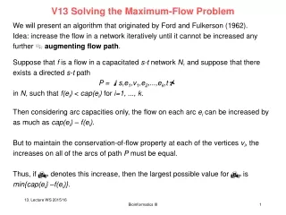
Algorithms for Max Flow • Sequential Algorithms • Ford and Fulkerson : Picks augmented paths arbitrarily • Edmonds and Karp : Use BFS to construct augmented paths • Goldmerg and Tarjan : Works in localized manner - O(ne log(n2/e)) • Parallel Algorithms • Shiloach and Vishkin : O(n2logn) using O(n) processors • Distributed Algorithms • Based mainly on the Glodmerg and Tarjan • Self-Stabilized Algorithms • Distributed Algorithms • Fault Tolerant • Adjust to dynamic changes in the network topology
Self-Stabilization • Introduced by Dijkstra [1974] • S is self-stabilizing with respect to predicate P if it satisfies the following two properties: • Closure: P is closed under the execution of S. • Convergence: Starting from an arbitrary global state, S is guaranteed to reach a global state satisfying P within a finite number of state transitions • Failure Model : Transient Failure • An event that may the change the state of the system, but not its behavior
Preliminaries • Skew Symmetry • Capacity Constraint • Residual Graph • Residual Capacity • Feasible flow • Max-flow, Min-cut theorem These terms are used in the same context
Model of Computation • Each node i in G corresponds to a process called process i that executes a program asynchronously • Each edge (i, j) corresponds to a bidirectional link b/w process i and process j • Process i local variables can be read by its neighbors but written only by process i • Program Model (expressed using guarded commands [Dijkstra 1975])
Maximum Flow Algorithm for Acyclic Graphs • G is a acyclic digraph • For each edge (i,j), f(i,j): current flow from node i to node j • Both process i and process j can read from and write into the variable f(i,j) • Each node i contains a single variable d(i): length of the shortest path form s to i in the residual graph Gf D(i): [0…n]
Key Idea… • For any node i , • Demand(i) = Of(i) – If(i) • Demand(t) = Infinity • Each node i tries to restore the flow conservation constraint demand(i)=0 by • Reducing its inflow if demand(i) < 0 • Increasing its inflow and or reducing its outflow if demand(i) > 0 • Each node with positive demand attempts to pull flow via a shortest path from s to itself in Gf • Use BFS to keep track of shortest paths from s to all nodes in Gf
Notation d = 4 c d = 3 b IN(i) = {a, b, c} D(i) = {4, 5, 6} d = 5 i a y d = 5 Residual Graph • Distinguished Nodes • Node s remains idle with d(s) = 0 • Node t executes the same program as other processes with demand(t) = INFINITY x
Algorithm • S1: Each node i, computes its d-value by examining the values d(j) for all (j,i)=Ef. d(i) = min{D[i], n} • S2: If demand(i)<0, then total flow along incoming edges in G is reduced irrespective of d-values • S3: if demand(i)>0 and d(i)<n, then i pulls flow along an incoming edges (j,i)=Ef and d(j)=d(i)-1 • S4: if demand(i) and d(i)=n, then there is no path from s to i in Gf and it reduces the outflow.
Algorithm • Assumption: f(i,j) never exceeds C(i,j) - New action (A5) that appropriately reduces the flow on an incident edge that has flow in excess of capacity
Example C(s,a) = C(b,t) = 2 C(a,b) = 1 Node: a Guard: S2 Node: b Guard: S1 Node: t Guard: S3 Node: b Guard: S3
Example … C(s,a) = C(b,t) = 2 C(a,b) = 1 Node: a Guard: S3 Node: b Guard: S1 Node: b Guard: S4 Node: t Guard: S1
Contribution of this paper • First distributed self-stabilizing algorithm for max-flow • Inherently tolerant to transient faults • Automatically adjust to topology changes • Arbitrary addition or deletion of edges • Addition and deletion of nodes provided that #nodes in the network is bounded • Arbitrary changes in the capacities of the edges • Requires O(n2) in average case settings