Probability

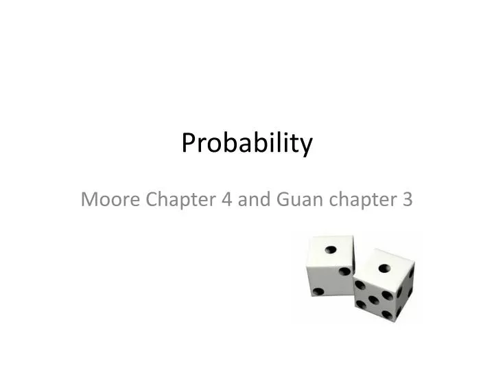
1. Probability Moore Chapter 4 and Guan chapter 3

2. Research questions • Play cards • Which is flower 2? • Say a number, and you do find the card with the number. What’s the probability?

3. Research questions • Parking strategy • If you want to park your car at the restrict area, what will you do to avoid the fine (if the policeman will patrol one street a day)? • Strategy A: park at the same place everyday? • Strategy B: change the place to park everyday?

4. Research questions • Why eastern society has more population in male? • Gene difference? • Society preference? • If yes, how does people birth more boys if they don’t kill kids? • Hepatitis B • Lin, Ming-Jen and Ming-Ching Luoh (2008), “Can Hepatitis B Mothers Account for the Number of Missing Women? Evidence from Three Million Newborns in Taiwan,” American Economic Review, 98:5, December, 2259-2273.

5. Randomness and probability Something like bar graph of relative frequency A phenomenon is random (隨機) if individual outcomes are uncertain, but there is nonetheless a regular distribution of outcomes in a large number of repetitions. The probability (機率) of any outcome of a random phenomenon can be defined as the proportion of times the outcome would occur in a very long series of repetitions.

6. Coin toss The result of any single coin toss is random. But the result over many tosses is predictable, as long as the trials are independent (i.e., the outcome of a new coin flip is not influenced by the result of the previous flip). The probability of heads is 0.5 = the proportion of times you get heads in many repeated trials. First series of tosses Second series

7. Two events are independent (獨立的) if the probability that one event occurs on any given trial of an experiment is not affected or changed by the occurrence of the other event. When are trials not independent? Imagine that these coins were spread out so that half were heads up and half were tails up. Close your eyes and pick one. The probability of it being heads is 0.5. However, if you don’t put it back in the pile, the probability of picking up another coin and having it be heads is now less than 0.5. The trials are independent only when you put the coin back each time. It is called sampling with replacement (取出放回抽樣).

8. Probability models • Probability models (機率模型) describe mathematically the outcome of random processes and consist of two parts: • 1) S = Sample Space (樣本空間, Ω): This is a set, or list, of all possible outcomes of a random process. An event (事件、集合) is a subset of the sample space. • 2) A probability for each possible event in the sample space S. Example: Probability Model for a Coin Toss: S = {Head, Tail} Probability of heads = 0.5 Probability of tails = 0.5

9. H - HHH H M - HHM H S = { HHH, HHM, HMH, HMM, MHH, MHM, MMH, MMM } Note: 8 elements, 23 H - HMH M M - HMM M … … Sample spacesIt’s the question that determines the sample space. A. A basketball player shoots three free throws. What are the possible sequences of hits (H) and misses (M)? B. A basketball player shoots three free throws. What is the number of baskets made? S = { 0, 1, 2, 3 }

10. Coin Toss Example: S = {Head, Tail} Probability of heads = 0.5 Probability of tails = 0.5 Probability rules 1) Probabilities range from 0 (no chance of the event) to1 (the event has to happen). For any event A, 0 ≤P(A) ≤ 1 Probability of getting a Head = 0.5 We write this as: P(Head) = 0.5 P(neither Head nor Tail) = 0 P(getting either a Head or a Tail) = 1 2) Because some outcome must occur on every trial, the sum of the probabilities for all possible outcomes (the sample space) must be exactly 1. P(sample space) = 1 Coin toss: S = {Head, Tail} P(head) + P(tail) = 0.5 + 0.5 =1  P(sample space) = 1

11. Coin Toss Example: S ={Head, Tail} Probability of heads = 0.5 Probability of tails = 0.5 Probability rules (cont.) 3) The complement (補集、餘集) of any event A is the event that A does not occur, written as Ac. The complement rule states that the probability of an event not occurring is 1 minus the probability that it does occur. P(not A) = P(Ac) = 1 −P(A) Tailc = not Tail = Head P(Tailc) = 1 − P(Head) = 0.5 Venn diagram: Sample space made up of an event A and its complementary Ac, i.e., everything that is not A.

12. Venn diagrams(范氏圖): A and B disjoint Probability rules (cont. ) 4) Two events A and B are disjoint (or said, mutually exclusive, 互斥事件) if they have no outcomes in common and can never happen together. The probability that A or B occurs is then the sum of their individual probabilities. Namely, the union (聯集) of two events is with probability: P(A or B) = “P(A U B)” = P(A) + P(B) This is the addition rule for disjoint events. A and B not disjoint Example:If you flip two coins, and the first flip does not affect the second flip: S = {HH, HT, TH, TT}. The probability of each of these events is 1/4, or 0.25. The probability that you obtain “only heads or only tails” is:P(HH or TT) = P(HH) + P(TT) = 0.25 + 0.25 = 0.50

13. Venn diagrams(范氏圖): A and B disjoint Probability rules (cont. ) 5) If two events A and B areNOT disjoint , then probability that A or B occurs is then the sum of their individual probabilities minus their intersection (交集). Namely, the union (聯集) of two events is with probability: P(A or B) = “P(A U B)” = P(A) + P(B) –P(A∩B) This is the addition rule for joint events. A and B not disjoint

14. Probability rules (cont. ) • Other probability rules • Commutative law (交換律) • A U B = B U A • A ∩ B=B ∩ A. • Associative law (結合律) • (A U B) U C = A U (B U C) • (A ∩ B) ∩ C = A ∩ (B ∩ C) • Distributive law (分配律) • A ∩ (B U C) = (A ∩ B) U (A ∩ C) • A U (B ∩ C) = (A U B) ∩ (A U C) • A ∩Ac=ϕ (空集合) • A UAc=Ω • De Morgan’s law (迪摩根定律) • (A U B)c=Ac ∩ Bc • (A ∩ B)c=Ac U Bc (A U B)c =Ac ∩ Bc A B (A ∩ B)c A B Try yourself!!

15. Probability rules (cont. ) • The probability of any random event A in sample space Ω must be satisfied: • P(A)≥0 • P(Ω)=1 • Fordisjoint (or said, mutually exclusive) events A1, A2, … • If • P(A ∩ B) is termed joint probability (聯合機率)

16. Assigning probabilities: finite number of outcomes Finite sample spaces deal with discrete data— data that can only take on a limited number of values. These values are often integers or whole numbers. The individual outcomes of a random phenomenon are always disjoint.  The probability of any event is the sum of the probabilities of the outcomes making up the event (addition rule). • Throwing a die: • S = {1, 2, 3, 4, 5, 6}

17. M&M’s candies If you draw an M&M’s candy at random from a bag, the candy will have one of six colors. The probability of drawing each color depends on the proportions manufactured, as described here: What is the probability that an M&M’s candy chosen at random is blue? S = {brown, red, yellow, green, orange, blue} P(S) = P(brown) + P(red) + P(yellow) + P(green) + P(orange) + P(blue) = 1 P(blue) = 1 – [P(brown) + P(red) + P(yellow) + P(green) + P(orange)] = 1 – [0.3 + 0.2 + 0.2 + 0.1 + 0.1] = 0.1 What is the probability that a random M&M’s candyis red, yellow, or orange? P(red or yellow or orange) = P(red) + P(yellow) + P(orange) = 0.2 + 0.2 + 0.1 = 0.5

18. Probabilities: equally likely outcomes We can assign probabilities either: • empirically  from our knowledge of numerous similar past events • Mendel (孟德爾) discovered the probabilities of inheritance of a given trait from experiments on peas (豌豆) without knowing about genes or DNA. • or theoretically  from our understanding the phenomenon and symmetries in the problem • A six-sided fair die: each side has the same chance of turning up • Genetic laws of inheritance based on meiosis process See details: http://zh.wikipedia.org/wiki/%E5%AD%9F%E5%BE%B7%E5%B0%94%E5%AE%9A%E5%BE%8B If a random phenomenon has k equally likely possible outcomes, then each individual outcome has probability 1/k. And, for any event A:

19. Dice You toss two dice. What is the probability of the outcomes summing to 5? This isS: {(1,1), (1,2), (1,3), ……etc.} There are 36 possible outcomes in S, all equally likely (given fair dice). Thus, the probability of any one of them is 1/36. P(the roll of two dice sums to 5) = P(1,4) + P(2,3) + P(3,2) + P(4,1) = 4 / 36 = 0.111

20. Dice • Or, you can solve the problem in this way: • Other questions: • The sum of outcomes could be divided by 3. • What is the probability for outcome of second dice is larger than the first outcome? • What is the probability for outcomes of two dices are the same? 6 5 4 3 2 1 1 2 3 4 5 6 • P=12/36=1/3 • P=(5+4+3+2+1)/36=15/36 • P=6/36=1/6

21. A couple wants three children. What are the arrangements of boys (B) and girls (G)? Genetics tell us that the probability that a baby is a boy or a girl is the same, 0.5. Sample space: {BBB, BBG, BGB, GBB, GGB, GBG, BGG, GGG} All eight outcomes in the sample space are equally likely. The probability of each is thus 1/8.  Each birth is independent of the next, so we can use the multiplication rule. Example: P(BBB) = P(B)* P(B)* P(B) = (1/2)*(1/2)*(1/2) = 1/8 A couple wants three children. What are the numbers of girls (X) they could have? The same genetic laws apply. We can use the probabilities above and the addition rule for disjoint events to calculate the probabilities for X. Sample space: {0, 1, 2, 3}P(X = 0) = P(BBB) = 1/8P(X = 1) = P(BBG or BGB or GBB) = P(BBG) + P(BGB) + P(GBB) = 3/8 …

22. Independence Two events are independent if the probability that one event occurs on any given trial of an experiment is not affected or changed by the occurrence of the other event. When are trials not independent? Imagine that these coins were spread out so that half were heads up and half were tails up. Close your eyes and pick one. The probability of it being heads is 0.5. However, if you don’t put it back in the pile, the probability of picking up another coin and having it be heads is now less than 0.5. The trials are independent only when you put the coin back each time. It is called sampling with replacement.

23. Multiplication rule for independent events Two events A and B are independent if knowing that one occurs does not change the probability that the other occurs. If A and B are independent, P(A and B) = P(A)P(B) This is the multiplication rule for independent events. Two consecutive coin tosses: P(first Tail and second Tail) = P(first Tail) * P(second Tail) = 0.5 * 0.5 = 0.25 Venn diagram: Event A and event B. The intersection represents the event {A and B} and outcomes common to both A and B.

24. Independent vs. disjoint events • Disjoint events are not independent. • If A and B are disjoint, then the fact that A occurs tells us that B cannot occur. So A and B are not independent. • Independence cannot be pictured in a Venn Diagram.

25. Applying the multiplication rule • If two events A and B are independent, the event that A does not occur is also independent of B. • The Multiplication Rule extends to collections of more than two events, provided that all are independent. • Example: A transatlantic data cable contains repeaters (中繼器) to amplify the signal. Each repeater has probability 0.999 of functioning without failure for 25 years. Repeaters fail independently of each other. Let A1 denote the event that the first repeater operates without failure for 25 years, A2 denote the event that the second repeater operates without failure for 25 years, and so on. The last transatlantic cable had 662 repeaters. The probability that all 662 will work for 25 years is: P(A1 and A2 and…and A662) = 0.999662 = 0.516

26. Applying the multiplication rule • If two events A and B are independent, the event that A does not occur is also independent of B. • The Multiplication Rule extends to collections of more than two events, provided that all are independent. • Example: The probability of positive result for one person is 0.2% or 0.002. What is the probability of at least one false positive drug test result occurring if 150 drug-free employees are tested?: P(single negative) = 1 – P(single positive) = 1 – 0.002 = 0.998 P(at least 1 positive) = 1 – P(no positives) = 1 – P(150 negatives) = 1 – (1 – 0.998)150 = 1 – 0.741 = 0.259

27. Conditional probability Conditional probabilities reflect how the probability of an event can change if we know that some other event has occurred/is occurring. • Example: The probability that a cloudy day will result in rain is different if you live in Los Angeles than if you live in Seattle. • Our brains effortlessly calculate conditional probabilities, updating our “degree of belief” with each new piece of evidence. The conditional probability of event B given event A is:(provided that P(A) ≠ 0)

28. Independent events Recall: A and B are independent when they have no influence on each other’s occurrence. • Two events A and B that both have positive probability are independent if P(B|A) = P(B). • The general multiplication rule then becomes: P(A and B) = P(A)P(B). • What is the probability of randomly drawing an ace of hearts from a deck of 52 playing cards? There are 4 aces in the pack and 13 hearts. • P(heart|ace) = 1/4 P(ace) = 4/52 • P(ace and heart) = P(ace)* P(heart|ace) = (4/52)*(1/4) = 1/52 Notice that heart and ace are independent events.

29. Tree diagram for chat room habits for three adult age groups 0.47 Internet user Tree diagrams Conditional probabilities can get complex, and it is often a good strategy to build a probability tree that represents all possible outcomes graphically and assigns conditional probabilities to subsets of events. P(chatting) = 0.136 + 0.099 + 0.017 = 0.252 About 25% of all adult Internet users visit chat rooms.

30. Baseball What is the probability of a high-school athlete playing professional baseball? P(B and A) = P(A)P(B | A) = (0.061)(0.094) = 0.00573 P(B and Ac) = P(A)P(B | Ac) = (0.939)(0.002) = 0.00188 P(B) = 0.00573 + 0.00188 = 0.00761 The probability of a high-school athlete playing in the MLB is about 0.8%.

31. Baseball What proportion of professional baseball players competed in college? P(A | B) = P(A and B)/P(B) = 0.00573/0.00761 = 0.753 About 75% of MLB players competed in college.

32. Diagnosis sensitivity 0.8 Disease incidence Positive Cancer 0.0004 False negative Negative 0.2 Mammography 0.1 False positive Positive 0.9996 No cancer Negative Incidence of breast cancer among women ages 20–30 0.9 Diagnosis specificity Mammography performance Breast cancer screening If a woman in her 20s gets screened for breast cancer and receives a positive test result, what is the probability that she does have breast cancer? She could either have a positive test and have breast cancer or have a positive test but not have cancer (false positive).

33. Diagnosis sensitivity Disease incidence Positive Cancer False negative Negative Mammography False positive Positive No cancer Negative Diagnosis specificity 0.8 0.0004 0.2 0.1 0.9996 Incidence of breast cancer among women ages 20–30 0.9 Mammography performance Possible outcomes given the positive diagnosis: positive test and breast cancer or positive test but no cancer (false positive). This value is called the positive predictive value, or PV+. It is an important piece of information but, unfortunately, is rarely communicated to patients.

34. Bayes’s rule An important application of conditional probabilities is Bayes’s rule. It is the foundation of many modern statistical applications beyond the scope of this textbook. * If a sample space is decomposed in k disjoint events, A1, A2, … , Ak— none with a null probability but P(A1) + P(A2) + … + P(Ak) = 1, * And if C is any other event such that P(C) is not 0 or 1, then: However, it is often intuitively much easier to work out answers with a probability tree than with these lengthy formulas.

35. Diagnosis sensitivity Disease incidence Positive Cancer False negative Negative Mammography False positive Positive No cancer Negative Diagnosis specificity If a woman in her 20s gets screened for breast cancer and receives a positive test result, what is the probability that she does have breast cancer? 0.8 0.0004 0.2 0.1 0.9996 Incidence of breast cancer among women ages 20–30 0.9 Mammography performance This time, we use Bayes’s rule: A1 is cancer, A2 is no cancer, C is a positive test result.