Download
1 / 39
390 likes | 657 Vues
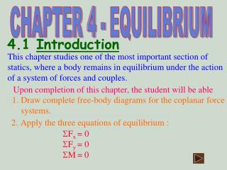
4.1 Introduction. 1. Draw complete free-body diagrams for the coplanar force systems. 2. Apply the three equations of equilibrium :. CHAPTER 4 - EQUILIBRIUM.

E N D
4.1Introduction 1. Draw complete free-body diagrams for the coplanar force systems. 2. Apply the three equations of equilibrium : CHAPTER 4 - EQUILIBRIUM This chapter studies one of the most important section of statics, where a body remains in equilibrium under the action of a system of forces and couples. Upon completion of this chapter, the student will be able Fx = 0 Fy = 0 M= 0
4.2 Equilibrium Newton’s First Law states that “ Every body remains at rest or maintains a constant velocity in a straight line unless an unbalanced force acts upon it. A body is said to be in equilibrium if the forces and moment acting on it are balanced, and the body remains at rest or, if it is in motion, there is no tendency for it to change its speed or direction. Hence for static equilibrium to occur: • Vertical forces must be balance; Fy = 0 • Horizontal forces must be balance; Fx = 0 • Moments must balance ie. ccw = cw; M= 0
4.3 Free-Body Diagrams (F.B.D.) Draw the object showing all the forces acting on it. • Start by drawing the body floating freely in space without any supports or connections like rollers, pinned joints etc. 2. Draw in all the known external applied forces on the body, and include the weight if given, acting vertically downwards from the centre of gravity (C.G) of the body. 3. Replace the supports or connections with the type of reaction forces on the body at these points (according to table 3.1 in the next slide) 4. Finally fill in information on slope angles,lengths or distances, etc for the analysis
F.B.D. Rc Frictionless Surface Table 3.1: Reactions at Various Types of Supports and Connections 1. Rollers Single reaction force at 90 0 to supporting surface
2. Cable & Short Link F.B.D. T Short Rope/ Cable Short Link Single force following direction of rope or link
3. Sliders Or Slot F.B.D. R 90o Frictionless Pin in Slot Slider on Frictionless Rod Single force at 90o to the guide (direction assumed)
F.B.D. or Fx R Fy Rough surface Frictionless pin or hinged joint Two components resolved into x and y axis or a single reaction of unknown direction 4. Hinged Joints
A 10 kN C B Example 4.1 Draw the free-body diagram for the lever ABC supported by roller at B and hinged at A as shown in the figure below.
A A 10 kN B C B Solution 4.1 • Draw the body ABC • (Remove all the supports) F.B.D. 2. Draw all applied loads Ay Ax 3. Draw the reaction forces at the supports. 10 kN Bx C
6 5 2 3 All dimensions in cm A 8 B E D 4 y 30kN C x Example 4.2 Draw free-body diagrams of the bar ABC and BDE as shown in the figure below. At A and D are pin joints, B is a slot and C is a smooth wall. (This example shows 2 objects connected via a slot at B)
Ay Ax 6 5 2 3 B A 8 Rc B 3 E 4 D 4 30kN C Solution 4.2 F.B.D. 1. Draw the body ABC 2. Draw the forces at the supports. A 9/3 = 3 12/3 = 4 Rb C
Rb 3 4 Dy 6 5 2 3 A 8 30 kN B E Dx D 4 30kN C 1. Draw the body BDE 2. Draw all applied loads F.B.D. 3. Draw the forces at the supports. E D B
= 0 = 0 4.4 Concurrent Force Systems When a system of forces intersect at a point (in the same plane) the system is known as the concurrent force system. To solve this we first draw a F.B.D. Next we apply the equations
Example 4.3 Two forces are in a state of equilibrium with a load of mass M kg as shown in the figure below. Determine the magnitude of force F and the mass M. F kN 5 kN y 60o 40o A x M kg
Solution 4.3 y F kN 5 kN 60o 40o x A L kN = 0 = 0 • Draw F.B.D. of point A 2. F Cos60o – 5 Cos40o = 0 (1) 3. F Sin60o + 5 Sin40o – M x 9.81 x 10-3 = 0 (2) From (1), F = 7.66 kN From (2), M x 9.81 x 10-3 = 7.66 Sin 60o + 5 Sin 40o = 9.85 kN M = (9.85/9.81) x 103 = 1004 kg
P P P P 4.5 Equilibrium of A Two Force Body Consider the body in the first figure above under the action of 2 forces. The body is not in equilibrium because there is a net moment. For equilibrium, the two forces must be equal and opposite so that the net force is zero and they must also act along the same line of action so that the net moment is also zero, as shown by the second figure. Equilibrium will be covered by Intermediate Mechanics in Level 2.
Body With 3 Forces F2 F2 F2 D D D F1 F1 d MD = 0, Not In Equilibrium F3 F3 F3 4.6 Equilibrium of A Three Force Body If a body is subjected to three forces at 3 points, for equilibrium, the vector sum of the components and the moments about any point must be zero. MD = 0, Fx = 0, Fy = 0, In Equilibrium
Example 4.4 A slender rod BC of length 2 m and weight 200 N is held by a cable AB and by a pin at C which slides in a vertical slot. Draw the free-body diagram of the rod BC. If is 30 0, determine the reaction at C, the angle and the tension in the cable AB. A Slot B C
y +ve 1 m x B 1 m Rc 30o C D E 200 N Solution 4.4 F.B.D. of ABC T
y +ve x 1 m B 1 m Rc 30o C D E 200 N Applying the moment equation at point B Mb = 0 (-200 x 1 x cos 30) + (Rc x 2 sin 30) = 0 Rc = 173.21 N To find , apply the Fx = 0 equation: T Fx = 0 Rc – T cos = 0, T cos = 173.21 (1)
y +ve x 1 m B 1 m Rc 30o C D E 200 N Fy = 0 T sin - 200 = 0, T sin = 200 (2) Equation (2) / (1), we get tan = 1.155 = 49.1 0 T And from (2) , T = 200/ sin = 264.6 N
a) b) c) 4.7 Equilibrium of Non-concurrent Multiple Force System Steps for solving problems 1. Draw Free-body Diagram 2. Apply the three Equations of Equilibrium (Take moment at pin joint)
Example 4.5 A light bar ABCD is hinged at B, supported by smooth roller at D is subjected to two forces as shown in the figure above. Find the reaction at B and D. 4m 1m 3m 65 0 B 480N D C A 50 0 200N
y +ve 4m 1m 3m x 65 0 B D C A Bx 50 0 By 480N Rd 200N Solution 4.5 F.B.D. of ABCD
4m 1m 3m 65 0 Apply at point B where there are 2 unknowns and note that the x-components of 480 N and 200 N passes through point B B 480N D C A Bx 50 0 Rd By 200N (Rd x 5) – (480 cos 65 x 4) + (200 sin 50 x 3) = 0 (Rd x 5) = 811.43 – 459.63 Rd = 70.36 N
4m 1m 3m 65 0 B 480N D C A Bx 50 0 Rd 200N By Bx = 306.47 N ( ) = 285.71 N ( ) Fx = 0, Bx + (480 sin 65) – 200 cos 50 = 0 Bx = (128.56 - 435.03) = - 306.47 N Applying Fy = 0, By + Rd – (480 cos 65) – (200 sin 50) = 0 By = (202.86 + 153.21 – 70.36) = + 285.71 N
Rb = ( Bx 2 + By 2) = 418.99 N Rb By Bx To find the magnitude and direction of the single reaction at B. Use vector addition for the Bx and By components: tan = (By / Bx) = (285.71 / 306.47) = 0.932 = 43.0 0 Rb = 418.99 N 43.0 0 = 43.0 0
C A G 2400 kg 1.5m B 2m 4m Example 4.6 A fixed crane has a mass of 1000 kg and is used to lift a 2400 kg crate. It is held in place by a pin at A and a roller at B. The center of gravity of the crane is located at G. Determine the components of the reactions at A and B.
y (1000 x g) N C Ay +ve A Ax x G (2400 x g) N 1.5m RB B 2m 4m Solution 4.6 F.B.D. of Crane
Apply RB = (160,884 / 1.5) = 107,256 N ( ) Ax = 107,256 N ( ) Ay = 33,354 N ( ) (RB x 1.5) – (1000 x 9.81 x 2) – (2400 x 9.81 x 6) = 0 C Ay Fx = 0 A Ax G Ax + RB = 0 (2400 x g) N 1.5m Ax = - 107,256 N RB (1000 x g) N B Fy = 0 2m 4m Ay – 1000 x 9.81 – 2400 x 9.81 = 0
300 N B 3 A C 4 D M kg 4.8 Pulleys Draw the F.B.D. of the pulley shown in the diagram below.
The tension in the cable is due to the 300 N force applied at one end of the cable. 300 N 300 N 3 Cx 4 Cy Since the cable has the same tension throughout its length, the free-body diagram of the pulley would have two forces of 300 N and the x and y-components at C.
If we apply the vector addition for the two 300 N forces, we obtain a resultant R = 537 N. Cx Cx R Cy Cy R=537 N For the system in equilibrium, the sum of moment at C must be zero and hence the resultant must pass through the point C.
300 N 300 N 300 N 3 Cx 4 300 N C R Cx 3 Cx Cy 4 Cy Cy Original system We can then resolve R back to the two original 300 N forces but now acting on the centre of the pulley, as shown below.
300N 300 N Ay 3 Ax C 4 D A (M x 9.81)N Hence for the example above, we could draw the following free-body diagrams, both of which are correct and the solution of either will yield the same answers for the reaction forces. When the pulley is drawn, the diameter of the pulley becomes insignificant. • With pulley
2) Without pulley 300N 300 N 3 Ay 4 Ax D A C (M x 9.81)N
F B 40o A C D 500 mm 700 mm 500 kg Example 4.7 A light bar AD is hinged at A and a pulley of diameter 3 cm is attached to the bar at C. It is held in horizontal position, with a load attached at D, by a force F applied via a rope attached at B and passing over pulley C. Draw the free-body diagram of the bar AD and determine the magnitude of the force F and the components of reaction at A.
y F F +ve 40o x Ay Ax C D A 0.5 m 0.7 m (500 x 9.81)N Solution 4.7 F.B.D. of bar AD
Apply F F Ay 40o Ax C D A 0.5 m 0.7 m Ax = 5492.01 N ( ) (500 x 9.81)N Ay = 6872.65 N ( ) (F x 0.5) + ( F sin 40 x 0.5) – (4905 x 1.2) = 0 0.5 F + 0.321 F = 5886 F =7,169.31 N Fx = 0 Ax +7169.31 Cos 40o = 0 Fy = 0 Ay + Fsin 40o – 4905 + F = 0